Page 1 Exposure Bracketing Exposure Bracketing capture additional - - PDF document

SLIDE 1

Page 1

Computational Photography Hendrik Lensch, Summer 2007

HDR, Demosaicing and Flash/No-flash imaging

Computational Photography Hendrik Lensch, Summer 2007

Projects

List available now Project proposal (2 pages): 1st of June Project idea presentation: 8th of June Final Project presentation: 20th of July Project report Persons to contact: me (228), Andrei Lintu (425), Tongbo Chen (221)

Computational Photography Hendrik Lensch, Summer 2007

Persons to contact

me (lensch@mpi-inf.mpg.de, room228) Andrei Lintu (lintu@mpi-inf.mpg.de, room 425) Tongbo Chen (tongbo@mpi-inf.mpg.de, room 221) Boris Ajdin (bajdin@mpi-inf.mpg.de, room 206) Matthias Hullin (hullin@mpi-inf.mpg.de, room 213)

Computational Photography Hendrik Lensch, Summer 2007

Metering

determine exposure time and aperture referenced to a standard 18% grey reflector incident light reflected light hand-held light meter

Computational Photography Hendrik Lensch, Summer 2007

In Camera Metering

inherent problem:

camera measures reflected light depends on object’s reflectance incident light reflected light

Computational Photography Hendrik Lensch, Summer 2007

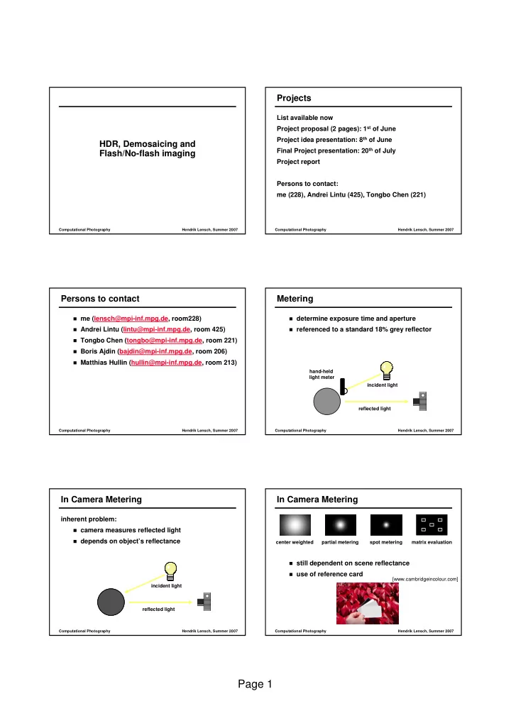
In Camera Metering

still dependent on scene reflectance use of reference card partial metering spot metering center weighted matrix evaluation [www.cambridgeincolour.com]

SLIDE 2

Page 2

Computational Photography Hendrik Lensch, Summer 2007

Exposure Bracketing

capture additional over and underexposed

images

Computational Photography Hendrik Lensch, Summer 2007

Exposure Bracketing

capture additional over and underexposed

images

Computational Photography Hendrik Lensch, Summer 2007

Exposure Bracketing

capture additional over and underexposed

images

how much variation? how to combine?

Computational Photography Hendrik Lensch, Summer 2007

Dynamic Range in Real World Images

natural scenes: 18 stops (2^18) human: 17stops

(after adaptation 30stops ~ 1:1,000,000,000)

camera: 10-16stops [Stumpfel et al. 00]

Computational Photography Hendrik Lensch, Summer 2007

Dynamic Range of Cameras

example: photographic camera with standard CCD sensor

• dynamic range of sensor

1:1000

• exposure variation (handheld camera/non-

static scene): 1/60th s – 1/6000th s exposure time 1:100

• varying aperture f/2.0 – f/22.0

~1:100

• exposure bias/varying “sensitivity”

1:10

• total (sequential)

1:100,000,000 simultaneous dynamic range still only 1:1000 similar situation for analog cameras

Computational Photography Hendrik Lensch, Summer 2007

High Dynamic Range (HDR) Imaging

basic idea of multi-exposure techniques:

combine multiple images with

different exposure settings

makes use of available

sequential dynamic range

• ther techniques available (e.g.

HDR video)

SLIDE 3

Page 3

Computational Photography Hendrik Lensch, Summer 2007

OECF Test Chart

absolute calibration

Computational Photography Hendrik Lensch, Summer 2007

High Dynamic Range Imaging

limited dynamic range of cameras is a problem

shadows are underexposed bright areas are overexposed sampling density is not sufficient

some modern CMOS imagers have a higher and

• ften sufficient dynamic range than most CCD

imagers

Computational Photography Hendrik Lensch, Summer 2007

High Dynamic Range (HDR) Imaging

analog film with several emulsions of different

sensitivity levels by Wyckoff in the 1960s

dynamic range of about 108

commonly used method for digital photography by

Debevec and Malik (1997)

selects a small number of pixels from the images performs an optimization of the response curve with a

smoothness constraint newer method by Robertson et al. (1999)

• ptimization over all pixels in all images

Computational Photography Hendrik Lensch, Summer 2007

High Dynamic Range Imaging

general idea of High Dynamic Range (HDR) imaging:

combine multiple images with different exposure

times

pick for each pixel a well exposed image response curve needs to be known don’t change aperture due to different depth-of-field

Computational Photography Hendrik Lensch, Summer 2007

High Dynamic Range Imaging

Computational Photography Hendrik Lensch, Summer 2007

HDR Imaging [Robertson et al.99]

Principle of this approach: Principle of this approach:

• calculate a HDR image using the response curve

calculate a HDR image using the response curve

• find a better response curve using the HDR image

find a better response curve using the HDR image (to be iterated until convergence) (to be iterated until convergence)

SLIDE 4

Page 4

Computational Photography Hendrik Lensch, Summer 2007

HDR Imaging [Robertson et al.99]

input:

series of i images with exposure times ti

and pixel values yij task:

find irradiance (luminance) xj recover response curve

) (

j i ij

x t f y =

ij

y j i ij

I x t y f = =

−

) (

1

) (

ij

y I

Computational Photography Hendrik Lensch, Summer 2007

HDR Imaging [Robertson et al.99]

input:

series of i images with exposure times ti and pixel

values yij

a weighting function wij = wij(yij) (bell shaped curve) a camera response curve

• initial assumption: linear response

⇒ calculate HDR values xj from images using

∑ ∑

=

i i ij i y i ij j

t w I t w x

ij

2

) (

ij

y I

Computational Photography Hendrik Lensch, Summer 2007

HDR Imaging [Robertson et al.99]

• ptimizing the response curve resp. :

minimization of objective function O

using Gauss-Seidel relaxation yields

normalization of I so that I128=1.0

2 ,

) (

j i j i y ij

x t I w O

ij −

=∑ } : ) , {( ) ( Card 1

,

m y j i E x t E I

ij m E j i j i m m

m

= = =

∑

∈

) (m I ) (

ij

y I

Computational Photography Hendrik Lensch, Summer 2007

HDR Imaging [Robertson et al.99]

both steps

calculation of a HDR image using I

• ptimization of I using the HDR image

are now iterated until convergence

criterion: decrease of O below some threshold usually about 5 iterations

Computational Photography Hendrik Lensch, Summer 2007

HDR Imaging [Robertson et al.99]

)) ( log(

ij

y I

Computational Photography Hendrik Lensch, Summer 2007

Example: Capturing Environment Maps

1/2000s 1/500s 1/125s 1/30s 1/2000s 1/500s 1/125s 1/30s 1/8s 1/8s series of input images series of input images

SLIDE 5

Page 5

Computational Photography Hendrik Lensch, Summer 2007

series of input images series of input images

Example: Capturing Environment Maps

Computational Photography Hendrik Lensch, Summer 2007

choice of weighting function w(yij) for response recovery

for 8 bit images possible correction at both ends

(over/underexposure)

motivated by general noise model

Weighting Function [Robertson et al.99]

        − − =

2 2

5 . 127 ) 5 . 127 ( 4 exp

ij ij

y w

Computational Photography Hendrik Lensch, Summer 2007

choice of weighting function w(yij) for HDR reconstruction

introduce certainty function c as derivative of the

response curve with logarithmic exposure axis

approximation of response function by cubic

spline to compute derivative

Weighting function [Robertson et al.03]

) ( ) (

ij

y ij ij

I c y w w = =

Computational Photography Hendrik Lensch, Summer 2007

Algorithm of Robertson et al.

consider response curve gradient what would be the best curve based on noise?

) ( ) (

ij

y ij ij

I c y w w = =

[Robertson et al. 2003]

Computational Photography Hendrik Lensch, Summer 2007

discussion

method very easy doesn’t make assumptions about response curve

shape

converges fast takes all available input data into account can be extended to >8 bit color depth 16bit should be followed by smoothing

Algorithm of Robertson et al.

Computational Photography Hendrik Lensch, Summer 2007

Input Images for Response Recovery

my favorite:

grey card, out of focus, smooth illumination

gradient advantages

uniform histogram of values no color processing or sharpening interfering

with the result

SLIDE 6

Page 6

Computational Photography Hendrik Lensch, Summer 2007

Input Images for HDR Generation

how many images are necessary to get good results?

depends on scene dynamic range and on quality

requirements

most often a difference of two stops (factor of 4)

between exposures is sufficient

[Grossberg & Nayar 2003]

Computational Photography Hendrik Lensch, Summer 2007

HDR-Video

LDR [Bennett & McMillan 2005] HDR image formats [OpenExr, HDR JPEG] HDR MPEG Encoding [Mantiuk et al. 2004] HDR + motion compensation [Kang et al. 2003]

Computational Photography Hendrik Lensch, Summer 2007

White Balance

daylight daylight flash flash flourescent flourescent tungsten tungsten

capture the spectral characteristics of the light source to assure correct color reproduction

Computational Photography Hendrik Lensch, Summer 2007

White Balance

build-in function derive scale from white point

sun incandescent tungsten infrared red green blue ultra violet wavelength Computational Photography Hendrik Lensch, Summer 2007

White Balance

build-in function derive scale from white point

infrared red green blue ultra violet wavelength Computational Photography Hendrik Lensch, Summer 2007

White Balance

build-in function derive scale from white point

infrared red green blue ultra violet wavelength

SLIDE 7

Page 7

Computational Photography Hendrik Lensch, Summer 2007

(ICC –international color consortium)

color management system capture the properties of all

devices

camera and lighting monitor settings

• utput properties

common interchange space sRGB standard as a definition

• f RGB

ICC Profiles

input device input device (e.g. camera) (e.g. camera) input profile input profile profile profile connection connection space space

• utput device
• utput device

(e.g. printer) (e.g. printer)

• utput profile
• utput profile

display display device device (e.g. (e.g. monitor) monitor) monitor monitor profile profile

Computational Photography Hendrik Lensch, Summer 2007

profile connection spaces

CIELAB (perceptual linear) linear CIEXYZ color space

can be used to create an high

dynamic range image in the profile connection space

allows for a color calibrated

workflow

ICC Profiles and HDR Image Generation

input device input device (e.g. camera) (e.g. camera) input profile input profile profile profile connection connection space space

• utput device
• utput device

(e.g. printer) (e.g. printer)

• utput profile
• utput profile

... ...

Computational Photography Hendrik Lensch, Summer 2007

3-Chip CCD

a prism splits up the incoming image into RGB

images

each color channel is captured by a different

sensor

registration during production problems with polarized light

Computational Photography Hendrik Lensch, Summer 2007

Color Wheel

• ne color channel is captured at one shot

3 times the acquisition time static images only

Computational Photography Hendrik Lensch, Summer 2007

Foveon Technology

3 layers capture RGB at the same location takes advantage of silicon’s wavelength

selectivity

light decays at different rates

for different wavelengths

multilayer CMOS sensor gets

3 different spectral sensitivities

don’t get to choose the curves

Computational Photography Hendrik Lensch, Summer 2007

Ways to sense color

Color filter array

paint each sensor with an individual filter requires just one chip but loses some spatial

resolution

“demosaicing” requires tricky image processing

primary secondary

SLIDE 8

Page 8

Computational Photography Hendrik Lensch, Summer 2007

take four images, moving the sensor by one pixel (use fourth image for noise reduction) can be used for supersampling

(move by ½, ¼ pixel)

Multi-Shot

Computational Photography Hendrik Lensch, Summer 2007

Demosaicing

Bilinear interpolation mosaic image [Alleysson & Suesstrunk05]

Computational Photography Hendrik Lensch, Summer 2007

Demosaicing

bilinear interpolation sampling theory edge-directed/pattern-based interpolation correlation-based

Computational Photography Hendrik Lensch, Summer 2007

Bilinear Interpolation

perform interpolation for each color channel separately

= + +

Computational Photography Hendrik Lensch, Summer 2007

Bilinear Interpolation

= + +

4

34 32 14 12 23

R R R R R + + + =

Computational Photography Hendrik Lensch, Summer 2007

Bilinear Interpolation

= + +

4

34 32 14 12 23

R R R R R + + + = 2

34 32 33

R R R + =

SLIDE 9

Page 9

Computational Photography Hendrik Lensch, Summer 2007

Bilinear Interpolation

set all non-measured values to zero then convolve

= + +

4 / 1 2 1 2 4 2 1 2 1

,

          =

B R

F 4 / 1 1 4 1 1           =

G

F

Computational Photography Hendrik Lensch, Summer 2007

Problem: Aliasing

[Alleysson & Suesstrunk05]

Computational Photography Hendrik Lensch, Summer 2007

Problem: Aliasing

[Alleysson & Suesstrunk05]

Computational Photography Hendrik Lensch, Summer 2007

Luminance and Chrominance

Luminance is sampled at every pixel Chrominance (opponent colors) only available on a sparser grid (zero mean)

• ne possible set for Bayer patterns:

)} , ( { ) , ( )} , ( { y x y x y x C I

i i

Ψ + Φ = = ) , ( ) , (

} , , {

y x C p y x

i B G R i i

∑

∈

= Φ

[Alleysson & Suesstrunk05]

∑

≠

− − = Ψ

i j j j i i i

y x C p y x C p y x ) , ( ) , ( ) 1 ( ) , (

low-pass high-pass

} 4 1 , 2 1 , 4 1 { = = =

B G R

p p p

Computational Photography Hendrik Lensch, Summer 2007

Fourier Space

/4 Computational Photography Hendrik Lensch, Summer 2007

Excessive Blurring

SLIDE 10

Page 10

Computational Photography Hendrik Lensch, Summer 2007

Grid Effect

Computational Photography Hendrik Lensch, Summer 2007

Watercolors

Computational Photography Hendrik Lensch, Summer 2007

False Color

Computational Photography Hendrik Lensch, Summer 2007

• ptimize r1 and r2 to gain best separation

Low-pass filter luminance High-pass filter chrominance (orthogonal filter) Demultiplex chrominance Interpolate opponent colors Add luminance and interpolated colors

[Alleysson & Suesstrunk05]

Computational Photography Hendrik Lensch, Summer 2007

Gradient-based (dcraw)

• 1. Calculate gradients in 5x5 region
• 2. Select subset of gradients (below threshold)
• 3. Average color differences in the determined regions

[Chuang et al. 99]

Computational Photography Hendrik Lensch, Summer 2007

Gradients

Gradient S =

+ − + − | 13 23 | | 8 18 | R R G G + − + − 2 / | 7 17 | 2 / | 9 19 | B B B B 2 / | 12 22 | 2 / | 14 24 | G G G G − + −

SLIDE 11

Page 11

Computational Photography Hendrik Lensch, Summer 2007

Regions

selection: gradient < 1.5*Min+0.5*(Max-Min) e.g. {S,W,NE,SE} S: R = (R13+R23)/2, G = G18, B = (B17+B19)/2 NE: R = (R13+R5)/2, G = (G4+G8+G10+G14)/4, B = B9 …

Computational Photography Hendrik Lensch, Summer 2007

Average

Rsum = (Rs + Rw + Rne + Rse)/4 Gsum = (Gs + Gw + Gne + Gse)/4 Bsum = (Bs + Bw + Bne + Bse)/4 average of color differences! G13 = R13 + (Gsum-Rsum); B13 = R13 + (Bsum-Rsum)

Computational Photography Hendrik Lensch, Summer 2007

Correlation-Based Demosaicing

Subband decomposition of full RGB-image using results in (LL, LH, HL, HH). Observation: inter channel correlation of red/green and blue/green is larger than 0.9. (discontinuities present in all channels at once!) => reconstruct (LH,HL,HH) for red and blue according to green

[Gunturk et al 02]

4 / ] 1 2 1 [ 4 / ] 1 2 1 [

1

− = = h h

Computational Photography Hendrik Lensch, Summer 2007

Alternating Projections

• 1. Interpolate red, green, and blue
• 2. Decompose all three channels (LL,HL,LH,HH)
• 3. Update red and blue high frequencies i=(HL,LH,HH)

according to green:

• 4. Reset observed data
• 5. Iterate: goto 2 until stopping criterion achieved.
• 6. Reconstruct image

i i i

green red r − =           − < − ≤ > + = T r T green T r red T r T green red

i i i i i i

; | | ; ;

Computational Photography Hendrik Lensch, Summer 2007

Comparison

gradient-selection correlation-based

Computational Photography Hendrik Lensch, Summer 2007

Comparison

gradient-selection correlation-based

SLIDE 12

Page 12

Computational Photography Hendrik Lensch, Summer 2007

Demosaicing – Take-home-points

2/3 of your image are just made up!

• avg. 5% error, much larger for individual pixels

color resolution is less than image resolution be careful with spiky BRDFs combining multiple video frames might help

Computational Photography Hendrik Lensch, Summer 2007

Flash-No-Flash [Eisenmann&Durand04]

[the following slides are from Eisenmann‘s SIGGRAPH talk]

Available light:

+ nice lighting

• noise/blurriness
• color

No-flash

Computational Photography Hendrik Lensch, Summer 2007

Flash

Flash:

+ details + color

• flat/artificial
• flash shadows
• red eyes

Flash

Computational Photography Hendrik Lensch, Summer 2007

Combined

Use no-flash image relight flash image

Flash No-flash Result

Computational Photography Hendrik Lensch, Summer 2007

Introduction

+ original lighting + details/sharpness + color Result No-flash

Use no-flash image relight flash image

Computational Photography Hendrik Lensch, Summer 2007

+

Blending

One approach: Blend the two photos

Introduction

No-flash Flash

SLIDE 13

Page 13

Computational Photography Hendrik Lensch, Summer 2007

Introduction

One approach: Blend the two photos

Blending [Eisenmann]

Computational Photography Hendrik Lensch, Summer 2007

One approach: Blend the two photos

Introduction

complex blending:

more details and less noise Blending [Eisenmann]

Computational Photography Hendrik Lensch, Summer 2007

Main Idea

Computational Photography Hendrik Lensch, Summer 2007

Structure

Computational Photography Hendrik Lensch, Summer 2007

Structure

Computational Photography Hendrik Lensch, Summer 2007

Intensity-Color Decomposition

Decomposition

SLIDE 14

Page 14

Computational Photography Hendrik Lensch, Summer 2007

Decomposition

Color / Intensity:

• riginal

= *

intensity color

Computational Photography Hendrik Lensch, Summer 2007

Frequency Decoupling

Decoupling

Computational Photography Hendrik Lensch, Summer 2007

Decoupling

Lighting : Large-scale variation Texture : Small-scale variation

Texture Lighting

Computational Photography Hendrik Lensch, Summer 2007

Large-scale Layer

Bilateral filter – edge preserving filter

Smith and Brady 1997; Tomasi and Manducci 1998; Durand et al. 2002

Input Output

Computational Photography Hendrik Lensch, Summer 2007

Large-scale Layer

Bilateral filter

Computational Photography Hendrik Lensch, Summer 2007

Detail Layer

Intensity Large-scale

/

=

Detail

Recombination: Large scale * Detail = Intensity

SLIDE 15

Page 15

Computational Photography Hendrik Lensch, Summer 2007

Recombination

Large-scale No-flash Detail Flash

*

Intensity Result

=

Recombination: Large scale * Detail = Intensity

Computational Photography Hendrik Lensch, Summer 2007

Recombination

Intensity Result Color Flash

~

*

~

Result

Recombination: Intensity * Color = Original shadows

Computational Photography Hendrik Lensch, Summer 2007

Results

Result No-flash Flash

Computational Photography Hendrik Lensch, Summer 2007

More Flash-noflash Algorithms

remove features that don’t appear in both (as determined from image gradients)

[following slides from Agrawal SIGGRAPH 2005]

Computational Photography Hendrik Lensch, Summer 2007 Computational Photography Hendrik Lensch, Summer 2007

SLIDE 16

Page 16

Computational Photography Hendrik Lensch, Summer 2007 Computational Photography Hendrik Lensch, Summer 2007 Computational Photography Hendrik Lensch, Summer 2007

Multi-Flash Images

extract edge information [following slides from Raskar 2004]

Computational Photography Hendrik Lensch, Summer 2007 Computational Photography Hendrik Lensch, Summer 2007 Computational Photography Hendrik Lensch, Summer 2007

SLIDE 17

Page 17

Computational Photography Hendrik Lensch, Summer 2007 Computational Photography Hendrik Lensch, Summer 2007 Computational Photography Hendrik Lensch, Summer 2007 Computational Photography Hendrik Lensch, Summer 2007 Computational Photography Hendrik Lensch, Summer 2007 Computational Photography Hendrik Lensch, Summer 2007

SLIDE 18

Page 18

Computational Photography Hendrik Lensch, Summer 2007 Computational Photography Hendrik Lensch, Summer 2007

Internal and external Shape boundaries, Occluding contour, Silhouettes

Depth Discontinuities

Computational Photography Hendrik Lensch, Summer 2007

Depth Edges

Depth Discontinuities

Computational Photography Hendrik Lensch, Summer 2007

Finding the Correct Edge

left flash right flash left/max right/max

Computational Photography Hendrik Lensch, Summer 2007

% Max composite maximg = max( left, right, top, bottom); % Normalize by computing ratio images r1 = left./ maximg; r2 = top ./ maximg; r3 = right ./ maximg; r4 = bottom ./ maximg; % Compute confidence map v = fspecial( 'sobel' ); h = v'; d1 = imfilter( r1, v ); d3 = imfilter( r3, v ); % vertical sobel d2 = imfilter( r2, h ); d4 = imfilter( r4, h ); % horizontal sobel %Keep only negative transitions silhouette1 = d1 .* (d1>0); silhouette2 = abs( d2 .* (d2<0) ); silhouette3 = abs( d3 .* (d3<0) ); silhouette4 = d4 .* (d4>0); %Pick max confidence in each confidence = max(silhouette1, silhouette2, silhouette3, silhouette4); imwrite( confidence, 'confidence.bmp');           − − − 1 1 2 2 1 1

Computational Photography Hendrik Lensch, Summer 2007

Multi-Flash Images

extract edge information

SLIDE 19

Page 19

Computational Photography Hendrik Lensch, Summer 2007

References - HDR

• M. A. Robertson, and R. L. Stevenson: Dynamic Range

Improvement through Multiple Exposures, IEEE ICIP, pp. 159-163, 1999.

• Mark A. Robertson, Sean Borman, and Robert L. Stevenson.

Estimation-Theoretic Approach to Dynamic Range Improvement Using Multiple Exposures. Journal of Electronic Imaging, 12(2),

• pp. 219-228, April 2003.
• M. D. Grossberg, S. K. Nayar: High Dynamic Range from Multiple

Images: Which Exposures to Combine? Proc. ICCV Workshop on Color and Photometric Methods in Computer Vision, 2003.

• R. Mantiuk, G. Krawczyk, K. Myszkowski, H.-P. Seidel:

Perception-Motivated High-Dynamic-Range Video Encoding, SIGGRAPH 2004.

• Sing Bing Kang, Matthew Uyttendaele, Simon Winder, Richard

Szeliski: High dynamic range video. ACM Transactions on Graphics (Proc. ACM SIGGRAPH 2003), 22 (3), pp. 319 – 325, 2003.

Computational Photography Hendrik Lensch, Summer 2007

References - Demosaicing

• D. Alleysson, S. Suesstrunk: Linear Demosaicing inspired by the

Human Visual System, IEEE Trans. on Image Processing, 14(4), 2005.

• B. K. Gunturk, Y. Altunbasak, R. M. Mersereau: Color Plane

Interpolation Using Alternating Projections, IEEE Trans. on Image Processing, 11(9), 2002.

• E. Chang, S. Cheung, D.Y. Pan: Color filter array recovery using a

threshold-based variable number of gradients. Proc. SPIE, vol. 3650, pp. 36-43, 1999.

• http://www-ise.stanford.edu/~tingchen/algodep/vargra.html

Computational Photography Hendrik Lensch, Summer 2007

References – Flash-No-Flash

• Flash photography enhancement via intrinsic relighting

Elmar Eisemann, Frédo Durand. ACM Transactions on Graphics. 23(3), pp. 673-678, 2004.

• Digital photography with flash and no-flash image pairs

Georg Petschnigg, Richard Szeliski, Maneesh Agrawala, Michael Cohen, Hugues Hoppe, Kentaro Toyama. ACM Transactions on Graphics. 23(3), pp. 664-672, 2004.

• Non-photorealistic camera: depth edge detection and stylized

rendering using multi-flash imaging Ramesh Raskar, Kar-Han Tan, Rogerio Feris, Jingyi Yu, Matthew Turk. ACM Transactions on Graphics. 23(3), pp. 679-688, 2004.

• Removing photography artifacts using gradient projection and

flash-exposure sampling Amit Agrawal, Ramesh Raskar, Shree K. Nayar, Yuanzhen Li. ACM Transactions on Graphics. 24(3), pp. 828-835, 2005.