A Look at the Alternative Minimum Tax Donald Bruce and Xiaowen Liu - PowerPoint PPT Presentation

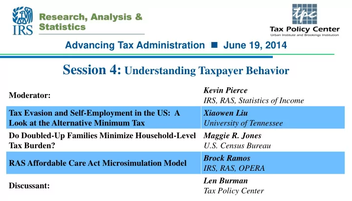
Advancing Tax Administration  June 19, 2014 Session 4: Understanding Taxpayer Behavior Kevin Pierce Moderator: IRS, RAS, Statistics of Income Tax Evasion and Self-Employment in the US: A Xiaowen Liu Look at the Alternative Minimum Tax University of Tennessee Do Doubled-Up Families Minimize Household-Level Maggie R. Jones Tax Burden? U.S. Census Bureau Brock Ramos RAS Affordable Care Act Microsimulation Model IRS, RAS, OPERA Len Burman Discussant: Tax Policy Center

Tax Evasion and Self-employment in the US: A Look at the Alternative Minimum Tax Donald Bruce and Xiaowen Liu Center for Business and Economic Research and Department of Economics The University of Tennessee, Knoxville IRS-TPC Research Conference June 19, 2014

Policy Background • The alternative minimum tax (AMT) for individuals is a separate income tax system in parallel to the regular income tax – Originally set to target high income individuals, AMT affects more middle income filers now – Taxpayers complete Form 6251 to find out if they owe the AMT, and how much they owe

Research Questions Do taxpayers manipulate their incomes in order to avoid the AMT as • they move toward the AMT threshold? If bunching is found, is there any difference between self-employed • individuals and wage earners? Does the behavioral response come from misreporting or real change • in activity? – If the response is driven by misreporting, the welfare loss is just or mainly tax revenue loss – If the response is partially driven by real activity, the welfare loss includes traditional excess burden, in addition to revenue loss

Previous Literature • Behavioral responses to the US income tax schedule: real response or misreporting? – Saez (2010) finds clear evidence of bunching by the EITC, and the bunching is concentrated among self-employed taxpayers – Kuka (2013) compares results from survey data and tax return data, and concludes that the bunching is mainly driven by misreporting • Related studies on behavioral responses to other programs – Ramnath (2013) – Chetty et. al. (2009) – Kleven and Waseem (2011)

Data • Individual Public Use Tax Files for 1994-2002 – limit our sample to those who filed Form 6251 – define the tax gap as the difference between the AMT liability and the regular tax liability Tax Gap = AMT Liability – Regular Tax Liability • This is not IRS defined tax gap • AMT is calculated based on tax return information on Form 1040 and Form 6251

Summary Statistics Variable Self-Employed Wage Earners 255,105.3 168,427.9 Adjusted Gross Income (median) 40,813.17 16,377.75 AMT Liability (median) 41,190 19,190 Regular Tax Liability (median) 0.14 0.27 Single (=1 if filed as single) 0.02 0.04 Head of Household (=1 if filed as head of household) 0.81 0.66 Married Filing Jointly (=1 if filed jointly) 0.02 0.03 Married Filing Separately(=1 if filed separately) 2.72 2.52 Total Number of Exemptions 9,023.1 2,552.0 State and Local Tax (median) – 4,302.8 – 2,887.4 Tax Gap (median) 0.23 0.27 % Pay AMT 100,198 20,290 Sample Size

Figure 1. Kernel Density of Tax Gap, 1994-2002

Figure 5. Tax Gap Distribution for the Self-employed and Wage Earners

Misreporting or Real Activity Response? • Expenditure-based approach by Pissarides and Weber (1989) • Tax-based consumption items on the Schedule A ( 𝑫 𝒋,𝒌 ) – Interest paid – Property tax paid – Charitable contributions 𝑫 𝒋,𝒌 𝒎𝒐 = 𝜸 𝟐 𝑼𝒃𝒚𝑯𝒃𝒒 𝒋,𝒌 + 𝜹 𝒋,𝒌 𝒂 𝒋,𝒌 + 𝒁𝒇𝒃𝒔 𝒌 + 𝝑 𝒋,𝒌 𝑼𝒑𝒖𝒃𝒎 𝑱𝒐𝒅𝒑𝒏𝒇

Results Variable ln (Interest Paid Ratio) ln (Property Tax Ratio) ln (Donation Ratio) 0.0000144*** 0.0000244*** 0.0000103*** Tax Gap (0.000003) (0.000002) (0.000003) The Self – employed 0.054* 0.024 0.260*** (0.031) (0.019) (0.029) The Self – employed *Tax Gap 0.000005* -0.000001 -0.00000704** (0.000003) (0.000002) (0.000003) -5.318*** -3.670*** -3.393*** Marginal Tax Rate (0.081) (0.052) (0.076) 0.0862*** 0.000612 0.0535*** Total Number of Exemptions (0.006) (0.004) (0.006) -0.035* 0.122*** 0.209*** Married Filing Jointly (0.021) (0.013) (0.019) -0.675*** 0.114*** 0.613*** Age 65 and Above (0.019) (0.011) (0.016) 60,203 67,452 68,441 Sample Size

Discussion • Evidence of misreporting – When tax gap increases, all three consumption ratios increase – The self-employed have higher ratio of tax consumption to income than wage earners – The self-employed appear to act more aggressively than wage earners when approaching the AMT threshold

Discussion • We find clear and significant behavioral responses to the AMT threshold • We find evidence of both real response and misreporting – Bunching among wage earners suggests real response – Consumption-based estimation suggests misreporting

Future Work • What we estimated can be interpreted as an upper bound of the behavioral response to the AMT • The results are all suggestive evidence because the data are pooled cross-section. Will need panel data to find causal effect. • Future work could continue the exploration of a causal impact of the AMT on taxpayer behavior if panel data is available

Thank you! Xiaowen Liu xliu23@utk.edu

Do Doubled-up Families Minimize Household-Level Tax Burden? Maggie R. Jones and Amy O’Hara U.S. Census Bureau IRS and Tax Policy Center: Joint 2014 Research Conference June 19, 2014 Disclaimer: This presentation is released to inform interested parties of ongoing research and to encourage discussion of work in progress. The views expressed on technical, statistical, or methodological issues are those of the author and not necessarily those of the U.S. Census Bureau.

Research question What predicts the sorting of dependent children, for tax purposes, between related adult filers in a household? Definitions  Sorting: There is a child in the household who  looks like he belongs to the reference person, according to survey response  is actually claimed by another adult relative in the household  Multiple related adult filers: A child, grandchild, parent, sibling, or other relative of a survey household reference person who lives in the HH and  files a 1040  is not claimed as a dependent on another return  Example: A mother with 2 children lives with her mother; the mom claims one child and the grandmother claims the other. 17

Mechanism  Income tax burden is  Unambiguously smaller for an individual when a dependent can be claimed  Larger or smaller for a household depending on the details of who claims or how many dependents each taxpayer claims  Complexity of income tax laws regarding qualifying children  Residency versus support  Relative status  Avoidance or evasion?  Complexity of rules leaves many situations open to interpretation  We assume sorting is generally allowed by rules (and we wouldn’t be able to distinguish anyway) 18

Incentives in Tax Rules  Dependent exemption  lowers taxable income for claimant  value depends on tax bracket  Head of household filing status  higher standard deduction  wider tax brackets  Earned Income Tax Credit (EITC)  Larger credits for more children, but  Credits are not multiplicative in children  Child Tax Credit (CTC, also ACTC)  Credit is per child 19

Example I: Single mother, single grandmother 20

Example II: Single mother, married grandmother 21

Model  Following McCubbin (2000), we use the increase in tax refund (or decrease in tax burden) due to optimal sorting of children: 𝜖𝐹(𝑧 𝑠 ,𝑦 𝑠 ) , 𝜖𝑦 𝑠 where 𝑧 𝑠 is reported income and 𝑦 𝑠 is number of claimed dependent children  For now, we express this in terms of EITC, which will make up much of the difference in burden  Using probit models, we use this value as the explanatory variable predicting whether or not a household sorts 22

Data  Current Population Survey Annual Social and Economic Supplement (CPS ASEC), 2006 – 2011  IRS tax data from 2005 – 2010  Universe of 1040s  Universe of W-2s  Records are matched at individual level using probability linkage techniques (Layne & Wagner, 2012)  Name, DOB, address, SSN used to assign unique identifier  Records linked using identifier, personal information stripped  Matches kept when CPS values not imputed 23

Eligibility modeling  Starting with relationship status in the CPS, modeling proceeds as in Jones (2013)  flag all eligible EITC units  calculate modeled credit amount  Sample selection  households with multiple adult related filers, and  households with at least one child claimed as a dependent on a tax return  all info on adult related filers then linked to the reference filer  We get original modeled totals for the household:  number of EITC-eligible filers  total credit amount  Simulated eligibility models are run (see next slide) 24

Simulated Eligibility  For every combination of filers/children in a household, we compute all possible EITC amounts for the household (up to a max of 3 filers and 6 children)  largest possible number of eligibility runs for a household is thus 28  all other variables that go into eligibility determination (income, earnings, etc.) remain the same  The simulated totals for the household are:  maximum number of EITC-eligible filers  maximum credit  We calculate the difference between original modeled credit and simulated maximum credit 25