
SLIDE 1
Page 1
Computational Photography Hendrik Lensch, Summer 2007
Optics
Computational Photography Hendrik Lensch, Summer 2007
Projects
List available now Project proposal (2 pages): 1st of June Project idea presentation: 8th of June Final Project presentation: 20th of July Project report
Computational Photography Hendrik Lensch, Summer 2007
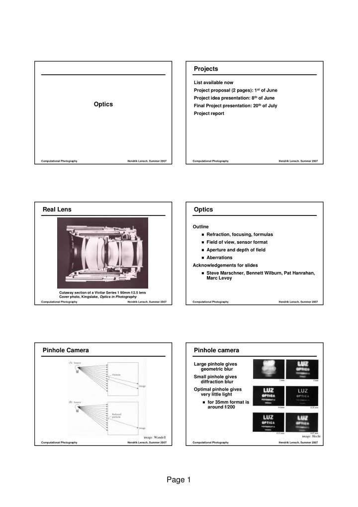
Real Lens
Cutaway section of a Vivitar Series 1 90mm f/2.5 lens Cover photo, Kingslake, Optics in Photography
Computational Photography Hendrik Lensch, Summer 2007
Optics
Outline
Refraction, focusing, formulas Field of view, sensor format Aperture and depth of field Aberrations
Acknowledgements for slides
Steve Marschner, Bennett Wilburn, Pat Hanrahan,
Marc Levoy
Computational Photography Hendrik Lensch, Summer 2007
Pinhole Camera
image: Wandell
Computational Photography Hendrik Lensch, Summer 2007
Pinhole camera
Large pinhole gives geometric blur Small pinhole gives diffraction blur Optimal pinhole gives very little light
for 35mm format is
around f/200
image: Hecht