Page 1 1 Review: Aliasing Review: Sampling Theorem and Nyquist - - PDF document

1

Page 1

University of British Columbia CPSC 314 Computer Graphics May-June 2005 Tamara Munzner http://www.ugrad.cs.ubc.ca/~cs314/Vmay2005

Scientific Visualization, Information Visualization I/II Week 5, Thu Jun 9

• News

P1 Hall of Fame take 2 P4 grading signup 12-4 Mon Jun 20

• Review: Image As Signal

1D slice of raster image discrete sampling of 1D spatial signal theorem any signal can be represented as an (infinite)

sum of sine waves at different frequencies

• Review: Summing Waves I

Review: Summing Waves II

represent spatial

signal as sum of sine waves (varying frequency and phase shift)

very commonly

used to represent sound “spectrum”

!

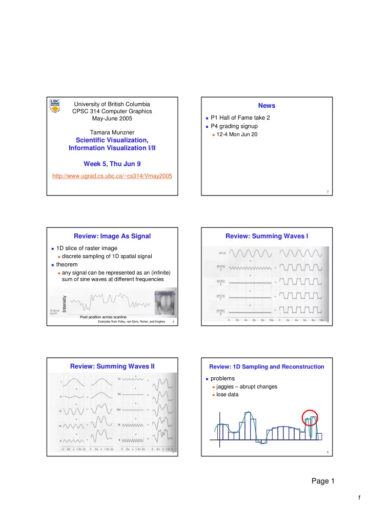
Review: 1D Sampling and Reconstruction

problems jaggies – abrupt changes lose data

2

Page 2

"

Review: Sampling Theorem and Nyquist Rate

Shannon Sampling Theorem

continuous signal can be completely recovered from

its samples iff sampling rate greater than twice maximum frequency present in signal

sample past Nyquist Rate to avoid aliasing

twice the highest frequency component in the

image’s spectrum

#

Review: Aliasing

incorrect appearance of high frequencies as

low frequencies

to avoid: antialiasing supersample

sample at higher frequency

low pass filtering

remove high frequency function parts aka prefiltering, band-limiting $

Review: Supersampling

%&

Review: Low-Pass Filtering

%%

Review: Invisible Primitives

why might a polygon be invisible?

polygon outside the field of view / frustum solved by clipping polygon is backfacing solved by backface culling polygon is occluded by object(s) nearer the viewpoint solved by hidden surface removal %

Review: Back-Face Culling

• n the surface of a closed orientable

manifold, polygons whose normals point away from the camera are always

• ccluded:

note: backface culling alone doesn’t solve the hidden-surface problem!

3

Page 3

%

Review: Painter’s Algorithm

draw objects from back to front problems: no valid visibility order for intersecting polygons cycles of non-intersecting polygons possible

%

Review: BSP Trees

preprocess: create binary tree recursive spatial partition viewpoint independent

%

Review: BSP Trees

runtime: correctly traversing this tree enumerates

• bjects from back to front

viewpoint dependent check which side of plane viewpoint is on at each node draw far, draw object in question, draw near

pros

simple, elegant scheme works at object or polygon level

cons

computationally intense preprocessing stage restricts

algorithm to static scenes

%!

Review: Warnock’s Algorithm

start with root viewport

and list of all objects

recursion:

clip objects to

viewport

if only 0 or 1 objects done else subdivide to new

smaller viewports

distribute objects to

new viewpoints

recurse %"

Review: Warnock’s Algorithm

termination viewport is single

pixel

explicitly check for

• bject occlusion

single-pixel case

common in high depth complexity scenes

%#

Review: Z-Buffer Algorithm

augment color framebuffer with Z-buffer or

depth buffer which stores Z value at each pixel

at frame beginning, initialize all pixel depths

to ∞

when rasterizing, interpolate depth (Z)

across polygon

check Z-buffer before storing pixel color in

framebuffer and storing depth in Z-buffer

don’t write pixel if its Z value is more distant

than the Z value already stored there

4

Page 4

%$

Review: Back-Face Culling

most objects in scene are typically “solid” rigorously: orientable closed manifolds

• rientable: must have two distinct sides

cannot self-intersect sphere is orientable boundary partitions space into interior & exterior Mobius strip or Klein bottle is not orientable do not partition space into interior & exterior closed: cannot “walk” from one side to other sphere is closed manifold, plane is not manifold: local neighborhood of all points

isomorphic to disc

Yes No No

&

Review: Back-face Culling

NDCS NDCS eye eye works to cull if works to cull if

>

Z

N

y y z z y y z z

<

Z

N

culling culling sometimes sometimes misses polygons that misses polygons that should be culled should be culled instead, cull if eye is instead, cull if eye is below polygon plane below polygon plane eye eye above above below below VCS VCS above above below below

%

Clarification/Review: Depth Test Precision

reminder: projective transformation maps

eye-space z to generic z-range (NDC)

thus zN ~= 1/zE

• ⋅
• −

− − − + − − + − − + − =

• E

E E E N N N N

w z y x n f fn n f n f b t b t b t n l r l r l r n w z y x 1 2 ) ( 2 2

E N E E N

z w w n f fn z n f n f z − = − − + − + − = , 2 ) (

E E N N

z w n f fn n f n f w z − + − + = 2

• Review: Rendering Pipeline

Geometry Database Geometry Geometry Database Database Model/View Transform. Model/View Model/View Transform. Transform. Lighting Lighting Lighting Perspective Transform. Perspective Perspective Transform. Transform. Clipping Clipping Clipping Scan Conversion Scan Scan Conversion Conversion Depth Test Depth Depth Test Test Texturing Texturing Texturing Blending Blending Blending Frame- buffer Frame Frame- buffer buffer

OCS OCS

• bject

WCS WCS world VCS VCS viewing CCS CCS clipping NDCS NDCS normalized device SCS SCS screen (2D) DCS DCS device (3D) (4D)

/w /w

• Scientific Visualization
• Reading

FCG Chapter 23

5

Page 5

• Surface Graphics
• bjects explicitly defined by surface or

boundary representation

mesh of polygons

200 polys 1000 polys 15000 polys

!

Surface Graphics

pros

fast rendering algorithms available hardware acceleration cheap OpenGL API for programming use texture mapping for added realism

cons

discards interior of object, maintaining only the shell

• perations such cutting, slicing & dissection not

possible

no artificial viewing modes such as semi-

transparencies, X-ray

surface-less phenomena such as clouds, fog & gas

are hard to model and represent

"

Volume Graphics

for some data, difficult to create polygonal mesh voxels: discrete representation of 3D object

volume rendering: create 2D image from 3D object

translate raw densities into colors and

transparencies

different aspects of the dataset can be emphasized

via changes in transfer functions

#

Volume Graphics

pros formidable technique for data exploration cons rendering algorithm has high complexity! special purpose hardware costly (~$3K-$10K) volumetric human head (CT scan)

$

Isosurfaces

2D scalar fields: isolines contour plots, level sets topographic maps 3D scalar fields: isosurfaces

&

Volume Graphics: Examples

anatomical atlas from visible human (CT & MRI) datasets industrial CT - structural failure, security applications flow around airplane wing shockwave visualization: simulation with Navier-Stokes PDEs

6

Page 6

%

Isosurface Extraction

array of discrete point

samples at grid points

3D array: voxels find contours closed, continuous determined by iso-value several methods marching cubes is most

common

• MC 1: Create a Cube

consider a cube defined by eight data values (i,j,k) (i+1,j,k) (i,j+1,k) (i,j,k+1) (i,j+1,k+1) (i+1,j+1,k+1) (i+1,j+1,k) (i+1,j,k+1)

• MC 2: Classify Each Voxel

classify each voxel according to whether lies

• utside the surface (value > iso-surface value)

inside the surface (value <= iso-surface value)

8

• 8

8 5 5 10 10 10

• MC 3: Build An Index

binary labeling of each voxel to create index v1 v2 v6 v3 v4 v7 v8 v5

• MC 4: Lookup Edge List

use index to access array storing list of edges all 256 cases can be derived from 15 base

cases

!

MC 4: Example

index = 00000001 triangle 1 = a, b, c

7

Page 7

"

MC 5: Interpolate Triangle Vertex

for each triangle edge find vertex location along edge using linear

interpolation of voxel values

• [ ]

[ ] [ ]

• −

+ − + = i v i v i v T i x 1

#

MC 6: Compute Normals

calculate the normal at each cube vertex use linear interpolation to compute the

polygon vertex normal

1 , , 1 , , , 1 , , 1 , , , 1 , , 1 − + − + − +

− = − = − =

k j i k j i z k j i k j i y k j i k j i x

v v G v v G v v G

$

MC 7: Render!

&

Direct Volume Rendering

do not compute surface

%

Rendering Pipeline

• Classification

data set has application-specific values temperature, velocity, proton density, etc. assign these to color/opacity values to make

sense of data

achieved through transfer functions

8

Page 8

• Transfer Functions

map data value to color and opacity

• Transfer Functions

Human Tooth CT

α α α α(f)

RGB(f)

f

RGB

shading, compositing…

α α α α

Gordon Kindlmann

• Setting Transfer Functions

can be difficult, unintuitive, and slow

f α f α f α f α

Gordon Kindlmann

!

Rendering Pipeline

• "

Light Effects

usually only consider reflected part

!"

# #$ #% !"#%&##&

!"

$ '# %%

s s d d a a

I k I k I k I + + =

!"$%%'#

#

Rendering Pipeline

9

Page 9

$

Interpolation

• !

( (

!

# !"# #

&

Rendering Pipeline

• %

Volume Rendering Algorithms

ray casting image order, forward viewing splatting

• bject order, backward viewing

texture mapping

• bject order

back-to-front compositing

• Ray Traversal Schemes

('" ) * +#! +$ ,#

• Ray Traversal - First

first: extracts iso-surfaces (again!)

('" ) ,#

• Ray Traversal - Average

average: looks like X-ray

('" ) +#!

10

Page 10

Ray Traversal - MIP

max: Maximum Intensity Projection used for Magnetic Resonance Angiogram

('" ) *

!

Ray Traversal - Accumulate

accumulate: make transparent layers visible

('" ) +$

"

Splatting

each voxel represented as fuzzy ball 3D gaussian function RGBa value depends on transfer function fuzzy balls projected on screen, leaving

footprint called splat

composite front to back, in object order

#

Texture Mapping

2D: axis aligned 2D textures

back to front compositing commodity hardware support must calculate texture

coordinates, warp to image plane

3D: image aligned 3D texture

simple to generate texture

coordinates