Page 1 1 Review: Marching Cubes Review: Direct Volume Rendering - - PDF document

1

Page 1

University of British Columbia CPSC 314 Computer Graphics May-June 2005 Tamara Munzner http://www.ugrad.cs.ubc.ca/~cs314/Vmay2005

Animation, Advanced Rendering, Final Review Week 6, Tue Jun 14

• News

P4 grading 4:30-5:45 Wed Jun 22

• Review: Volume Graphics

for some data, difficult to create polygonal mesh voxels: discrete representation of 3D object

volume rendering: create 2D image from 3D object

translate raw densities into colors and

transparencies

different aspects of the dataset can be emphasized

via changes in transfer functions

• Review: Volume Graphics

pros formidable technique for data exploration cons rendering algorithm has high complexity! special purpose hardware costly (~$3K-$10K) volumetric human head (CT scan)

• Review: Isosurfaces

2D scalar fields: isolines contour plots, level sets topographic maps 3D scalar fields: isosurfaces

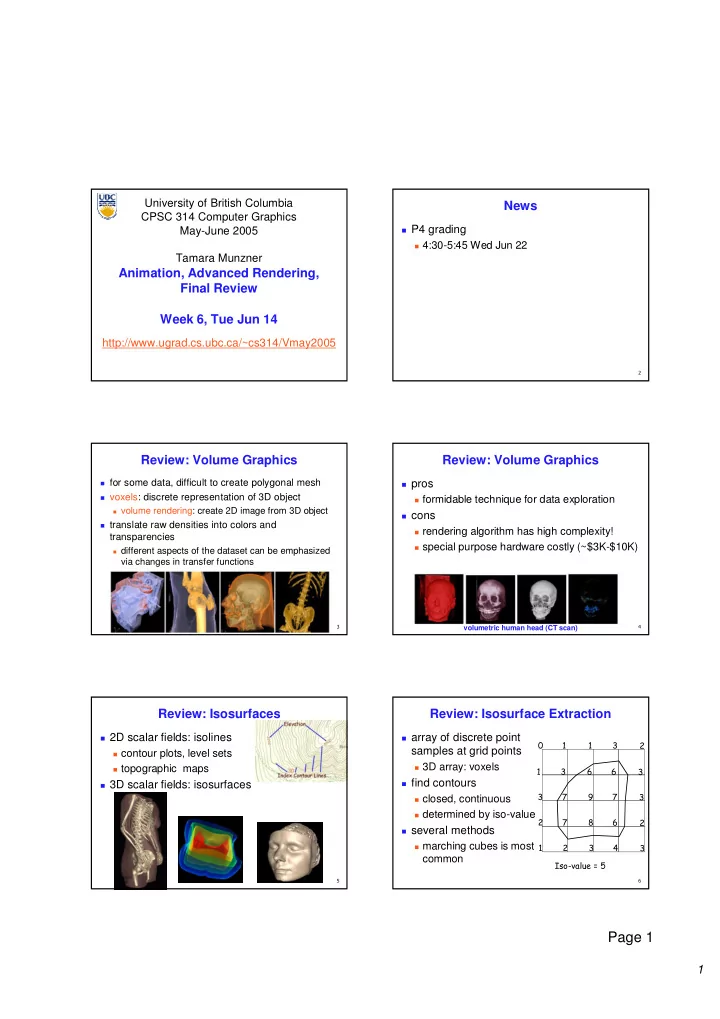
• Review: Isosurface Extraction

array of discrete point

samples at grid points

3D array: voxels find contours closed, continuous determined by iso-value several methods marching cubes is most

common

2

Page 2

• Review: Marching Cubes

create cube classify each voxel binary labeling of each voxel to

create index

use in array storing edge list all 256 cases can be derived

from 15 base cases

interpolate triangle vertex calculate the normal at each

cube vertex

render by standard methods

• Review: Direct Volume Rendering Pipeline
• do not compute surface
• Review: Transfer Functions To Classify

map data value to color and opacity can be difficult, unintuitive, and slow

f α f α f α f α

Gordon Kindlmann

• Review: Volume Rendering Algorithms

ray casting image order, forward viewing splatting

• bject order, backward viewing

texture mapping

• bject order

back-to-front compositing

• Review: Ray Casting Traversal Schemes
• !

""# $

• Review: Information Visualization

interactive visual representation of abstract data

help human perform some task more effectively

bridging many fields

graphics: interacting in realtime cognitive psych: finding appropriate representation HCI: using task to guide design and evaluation

external representation

reduces load on working memory

• ffload cognition

familiar example: multiplication/division infovis example: topic graphs

3

Page 3

• Review: Shneiderman mantra
• verview, zoom and filter, details-on-demand
• Review: Overviews - SeeSoft

colored lines of code: lines one pixel high

• Review: Focus+Context

integrate overview and details into single view

H3: 3D fisheye TreeJuxtaposer: stretch and squish SpaceTree: collapse/expand

• Review: 3D Extrusion vs. Linking

perspective interferes with comparison daily, weekly patterns hard to see linked cluster/calendar view more effective [van Wijk and van Selow, Cluster and Calendar based Visualization of Time Series Data, InfoVis99, citeseer.nj.nec.com/vanwijk99cluster.html]

• Review: Preattentive Visual Channels: Popout

single channel processed in parallel for popout

visual attentional system not invoked speed independent of distractor count hue, shape, texture, length, width, size, orientation,

curvature, intersection, intensity, flicker, direction of motion, stereoscopic depth, lighting direction,...

multiple channels not parallel

search linear in number of

distractor objects

[Chris Healey, Preattentive Processing, www.csc.ncsu.edu/faculty/healey/PP]

• Review: Data Type Affects Channel Ranking

spatial position best for all types

accuracy at judging magnitudes, from best to worst [Mackinlay, Automating the Design of Graphical Presentations of Relational Information, ACM TOG 5:2, 1986] [Card, Mackinlay, and Shneiderman. Readings in Information Visualization: Using Vision to Think. Morgan Kaufmann 1999. Chapter 1]

4

Page 4

• Review: Coloring Categorical Data

discrete small patches separated in space limited distinguishability: around 8-14 channel dynamic range: low choose bins explicitly for maximum mileage maximally discriminable colors from Ware maximal saturation for small areas

• vs. minimal saturation for large areas

[Colin Ware, Information Visualization: Perception for Design. Morgan Kaufmann 1999. Figure 4.21]

• Review: Rainbow Colormap Disadvantages

perceptually nonlinear segmentation, hue unordered (partial) solution perceptually isolinear map [Kindlmann, Reinhard, and Creem. Face-based Luminance Matching for Perceptual Colormap Generation.

• Proc. Vis 02 www.cs.utah.edu/~gk/lumFace]

[Rogowitz and Treinish, How NOT to Lie with Visualization,www.research.ibm.com/dx/proceedings/pravda/truevis.htm

• Review: Color Deficiency – vischeck.com

10% of males have red/green deficit

• Review: Space vs. Time: Showing Change
• Review: Space vs. Time: Showing Change
• Animation

(slides based on Robert Bridson’s CPSC 426 preview) www.ugrad.cs.ubc.ca/~cs426

5

Page 5

• Computer Animation
• ffline: generate a film, play it back later

long ago reached the point of being able to

render anything an artist could model

problem is: how to model? tools/UI for directly specifying model+motion

(the traditional technique)

procedural modeling (e.g. particle systems) data-driven modeling (e.g. motion capture) physics-based modeling (e.g. fluid simulation)

• Real-Time Animation

for example, games rendering limited, modeling even more limited “traditional” technique - replay scripted

motions

but scalability/realism are becoming a problem need to generate more new motion on the fly

• Traditional CG Animation

Grew out of traditional animation [Pixar] every detail of every model is parameterized

e.g. position and orientation of base of lamp, joint

angles, lengths, light intensity, control points for spline curve of power cord, …

associate a “motion curve” with each parameter -

how it changes in time

animating == designing motion curves

• Motion Curves

keyframe approach:

artist sets extreme values at important frames computer fills in the rest with splines artist adjusts spline controls, slopes, adds more

points, adjusts, readjusts, re-readjusts, …

straight-ahead approach:

artist simply sets parameters in each successive

frame

layering approach:

design the basic motion curves first, layer detail on

afterwards

• Motion Curve Tools

retiming: keep the shape of the trajectory, but

change how fast we go along it

add a new abstract motion curve controlling

distance traveled along trajectory

Inverse Kinematics (IK): given a skeleton (specified by joint angles) artist directly controls where parts of the

skeleton go, computer solves for the angles that achieve that

• Procedural Modeling

write programs to automatically generate models

and motion

for example, “flocking behaviour” build a flock of birds by specifying simple rules of

motion:

accelerate to avoid collisions accelerate to fly at preferred distance to nearby birds accelerate to fly at same velocity as nearby birds accelerate to follow “migratory” impulse

let it go, hope the results look good

6

Page 6

• Data-Driven Modeling

measure the real world, use that data to

synthesize models

laser scanners camera systems for measuring reflectance

properties

Image-Based Rendering - e.g. Spiderman …

• Data-Driven Motion

record real motion (motion capture = mocap) then play it back but life is never that simple real motion is hard to measure measurements are noisy won’t quite fit what you needed not obviously adaptable to new environments,

interactive control, etc.

• Marker-Based Mocap

stick performer in a tight black suit, stick

markers on body, limbs, …

film motion with an infrared strobe light and

multiple calibrated cameras

reconstruct 3D trajectories of markers, filling

in gaps and eliminating noise

infer motion of abstract skeleton clean up data drive CG skeleton with recorded motion

curves

• What it looks like…

(from Zoran Popovic’s website)

• Footskate and Clean Up

most common problem: footskate feet that in reality were stuck to floor hover

and slip around

fix using IK: determine target footplants,

automatically adjust joint angles to keep feet planted

• ften OK to even adjust limb lengths…
• Motion Control

how do you adapt mocap data to new

purposes?

motion graphs (remixing) motion parameterization (adjust mocap data) motion texturing (add mocap details to

traditional animation)

7

Page 7

• Motion Graphs

chop up recorded data into tiny clips aim to cut at common poses build graph on clips: connect two clips if the

end pose of one is similar to the start pose of another

then walk the graph figure out smooth transitions from clip to clip navigate a small finite graph instead of infinite

space of all possible motions

• Physics-based modeling

like procedural modeling, only based on laws of

physics

if you want realistic motion, simulate reality human motion:

specify muscle forces (joint torques), simulate actual

motion

has to conserve momentum etc. can handle the unexpected (e.g. a tackle) but need to write motion controllers

passive motion:

figure out physical laws behind natural phenomena simulate (close cousin of scientific computing)

• Advanced Rendering
• Reading

FCG Chapter 9: Ray Tracing

• nly 9.1-9.7

FCG Chap 22: Image-Based Rendering

• Errata

p 155

line 1: p(t)=e+td, not p(t)=o+td equation 5: 2nd term 2d*(e-c), not 2d*(o-e)

p 157

matrices: cx->xc, cy->yc, cz->zc

p 162

r = d – 2(d.n)n, not r = d + 2(d.n)n

p 163

eqn 4 last term: n cos θ not n cos θ ’ eqn 5: no θ term at end

• Global Illumination Models

simple shading methods simulate local

illumination models

no object-object interaction global illumination models more realism, more computation approaches ray tracing subsurface scattering radiosity

8

Page 8

• Simple Ray Tracing

view dependent method cast a ray from viewer’s

eye through each pixel

compute intersection of

ray with first object in scene

cast ray from

intersection point on

• bject to light sources

projection reference point pixel positions

• n projection

plane

• Recursive Ray Tracing

ray tracing can handle

reflection (chrome) refraction (glass) shadows

spawn secondary rays

reflection, refraction if another object is hit,

recurse to find its color

shadow cast ray from intersection

point to light source, check if intersects another object

projection reference point pixel positions

• n projection

plane

• Reflection

mirror effects

perfect specular reflection

n

θ θ

• Refraction

happens at interface

between transparent object and surrounding medium

e.g. glass/air boundary

Snell’s Law

• light ray bends based on

refractive indices c1, c2

2 2 1 1

sin sin θ θ c c =

n

θ 1 θ 2

d t

• Total Internal Reflection

http://www.physicsclassroom.com/Class/refrn/U14L3b.html

• Ray Tracing Algorithm

Whitted, 1980 Image Plane Light Source Eye Refracted Ray Reflected Ray Shadow Rays

9

Page 9

• Basic Ray Tracing Algorithm

RayTrace(r,scene)

• bj := FirstIntersection(r,scene)

if (no obj) return BackgroundColor; else begin if ( Reflect(obj) ) then reflect_color := RayTrace(ReflectRay(r,obj)); else reflect_color := Black; if ( Transparent(obj) ) then refract_color := RayTrace(RefractRay(r,obj)); else refract_color := Black; return Shade(reflect_color,refract_color,obj); end;

• Algorithm Termination Criteria

termination criteria no intersection reach maximal depth

number of bounces

contribution of secondary ray attenuated

below threshold

each reflection/refraction attenuates ray

• Ray - Object Intersections

inner loop of ray-tracing must be extremely efficient solve a set of equations ray-sphere ray-triangle ray-polygon

• Ray - Sphere Intersection

ray: unit sphere: quadratic equation in t:

x t p v t y t p v t z t p v t

x x y y z z

( ) , ( ) , ( ) = + = + = +

p v

x y z

2 2 2

1 + + =

1 2 1

2 2 2 2 2 2 2 2 2 2

= + + + + + − = + + + + + + + + − ( ) ( ) ( ) ( ) ( ) ( ) p v t p v t p v t t v v v t p v p v p v p p p

x x y y z z x y z x x y y z z x y z

• Optimized Ray-Tracing

basic algorithm simple but very expensive

• ptimize by reducing:

number of rays traced number of ray-object intersection calculations methods bounding volumes: boxes, spheres spatial subdivision

uniform BSP trees

(not required reading)

• Subsurface Scattering: Translucency

light enters and leaves at different locations

• n the surface

bounces around inside technical Academy Award, 2003 Jensen, Marschner, Hanrahan

10

Page 10

• Subsurface Scattering: Marble
• Subsurface Scattering: Milk vs. Paint
• Subsurface Scattering: Faces
• Subsurface Scattering: Faces
• Radiosity

radiosity definition

rate at which energy emitted or reflected by a surface

radiosity methods

capture diffuse-diffuse bouncing of light indirect effects difficult to handle with raytracing

• Radiosity

recall radiative heat transfer

conserve light energy in a volume model light transport until convergence solution captures diffuse-diffuse bouncing of light

view independent technique

calculate solution for entire scene offline browse from any viewpoint in realtime

heat/light source thermometer/eye reflective objects energy packets

11

Page 11

• Radiosity

[IBM] [IBM]

divide surfaces into small patches loop: check for light exchange between all pairs

form factor: orientation of one patch wrt other patch (n x n matrix)

• Raytracing vs. Radiosity Comparison

ray-tracing: great specular, approx. diffuse view dependent radiosity: great diffuse, specular ignored view independent, mostly-enclosed volumes advanced hybrids: combine them

raytraced radiosity

• Image-Based Rendering

store and access only pixels no geometry, no light simulation, ... input: set of images

• utput: image from new viewpoint

surprisingly large set of possible new viewpoints

• IBR Characteristics

display time not tied to scene complexity expensive rendering or real photographs massive compression possible (120:1) can point camera in or out QuickTimeVR: camera rotates, no translation

• Characterizing Light

7D plenoptic function: P(x, y, z, θ, φ, λ, t) (x,y,z): every position in space (θ, φ): every angle λ: every wavelength of light t: every time can simplify to 4D function fix time: static scene fix wavelength: static lighting partially fix position: empty space between

camera and object

• 4D Light Field / Lumigraph

P(u,v,s,t) images: just one kind of 2D slice

12

Page 12

• Non-Photorealistic Rendering

look of hand-drawn sketches or paintings

www.red3d.com/cwr/npr/

• NPRQuake

www.cs.wisc.edu/graphics/Gallery/NPRQuake/

• Advanced Rendering

so many more algorithms, so little class time! Renderman REYES photon mapping and lots more...

• Final Review
• Final Logistics

12:0pm-2:30pm Thu Jun 16 here (MCLD 202) notes: both sides 8.5”x11” handwritten page calculator OK if you want have photo ID face up on desk spread out, sit where there is an exam

• Reading from OpenGL Red Book

1: Introduction to OpenGL 2: State Management and Drawing Geometric Objects 3: Viewing 4: Display Lists 6: Lighting 9: Texture Mapping 12: Selection and Feedback 13: Now That You Know

• nly section Object Selection Using the Back Buffer

Appendix: Basics of GLUT (Aux in v 1.1) Appendix: Homogeneous Coordinates and Transformation

Matrices

13

Page 13

• Reading from Shirley: Foundations of CG

2: Misc Math 3: Raster Algs except for 3.8 4: Linear Algebra

• nly 4.1-4.2.5

5: Transforms except 5.1.6 6: Viewing 7: Hidden Surfaces 8: Surface Shading 9: Ray Tracing

• nly 9.1-9.7

10: Texture Mapping 11: Graphics Pipeline

• nly 11.1-11.4

12: Data Structures

• nly 12.3

13: Curves and Surfaces 17: Human Vision 18: Color

• nly 18.1-18.8

22: Image-Based Rendering 23: Visualization

• Studying Advice

do problems! work through old homeworks, exams

• Midterm Topics Covered

rendering pipeline projective rendering pipeline

coordinate systems

transformations viewing projections

• Review: Rendering Pipeline

pros and cons of pipeline approach Geometry Database Geometry Geometry Database Database Model/View Transform. Model/View Model/View Transform. Transform. Lighting Lighting Lighting Perspective Transform. Perspective Perspective Transform. Transform. Clipping Clipping Clipping Scan Conversion Scan Scan Conversion Conversion Depth Test Depth Depth Test Test Texturing Texturing Texturing Blending Blending Blending Frame- buffer Frame Frame- buffer buffer

• Review: Projective Rendering Pipeline

OCS - object coordinate system WCS - world coordinate system VCS - viewing coordinate system CCS - clipping coordinate system NDCS - normalized device coordinate system DCS - device coordinate system

OCS OCS WCS WCS VCS VCS CCS CCS NDCS NDCS DCS DCS

modeling modeling transformation transformation viewing viewing transformation transformation projection projection transformation transformation viewport viewport transformation transformation alter w alter w / w / w

• bject

world viewing/ camera device normalized device clipping

perspective perspective division division glVertex3f(x,y,z) glVertex3f(x,y,z) glTranslatef(x,y,z glTranslatef(x,y,z) ) glRotatef(th,x,y,z glRotatef(th,x,y,z) ) .... .... gluLookAt gluLookAt(...) (...) glFrustum glFrustum(...) (...) glutInitWindowSize(w,h glutInitWindowSize(w,h) ) glViewport(x,y,a,b glViewport(x,y,a,b) )

• Review: Transformations, Homog. Coords
• =
• 1

1 1 1 1 1 ' ' ' z y x c b a z y x translate(a,b,c) translate(a,b,c)

• −

=

• 1

1 cos sin sin cos 1 1 ' ' ' z y x z y x θ θ θ θ

) , ( Rotate θ x

• =
• 1

1 1 ' ' ' z y x c b a z y x scale(a,b,c) scale(a,b,c)

• −

1 cos sin 1 sin cos θ θ θ θ

) , ( Rotate θ y

• −

1 1 cos sin sin cos θ θ θ θ

) , ( Rotate θ z y y w w w= w=1 1

• ⋅

⋅ w w y w x

• ⋅

⋅ w w y w x

• 1

y x

• 1

y x

14

Page 14

• Review: Transforming View Volumes

x z

NDCS

y

(-1,-1,-1) (1,1,1)

• rthographic view volume
• rthographic view volume

x z VCS y x=left y=top x=right z=-far z=-near y=bottom perspective view volume perspective view volume x=left x=right y=top y=bottom z=-near z=-far x VCS y

• Review: Basic Perspective Projection

similar triangles similar triangles

→ = z y d y' z d y y ⋅ = '

z z P(x,y,z) P(x,y,z) P(x’,y’,d P(x’,y’,d) ) z=d z=d y y also also

z d x x ⋅ = '

nonuniform foreshortening not affine

d z = '

but but

• Post-Midterm Topics Covered

rasterization interpolation/bary coords color lighting shading compositing clipping curves picking collision textures procedural approaches sampling virtual trackball visibility scientific visualization information visualization advanced rendering animation

• Review: Rasterization

lines: midpoint algorithm

• ptimized: Bresenham

polygons flood fill scanline algorithms parity test for general case

1 2 3 4 5=0 P

• Review: Barycentric Coordinates

weighted combination of vertices 3 2 1

P P P P ⋅ + ⋅ + ⋅ = γ β α

1

P

3

P

2

P P

(1,0,0) (1,0,0) (0,1,0) (0,1,0) (0,0,1) (0,0,1)

5 . = β 1 = β = β 1 , , 1 ≤ ≤ = + + γ β α γ β α

“ “convex combination convex combination

• f points”
• f points”
• Review: Color

color perception

color is combination of

stimuli from 3 cones

metamer: identically

perceived color caused by very different spectra

simple model: based on

RGB triples

component-wise

multiplication of colors

(a0,a1,a2) * (b0,b1,b2) =

(a0*b0, a1*b1, a2*b2)

15

Page 15

• Review: Lighting

Idiffuse = kd Ilight (n • l)

n l θ R = 2 ( N (N · L)) – L

Ispecular = ksIlight(v•r)nshiny

Itotal = ksIambient + Ii(

i=1 # lights

• kd(n•li) + ks(v•ri)nshiny )

reflection equations full Phong lighting model combine ambient, diffuse, specular components

• Review: Shading Models

flat shading compute Phong lighting once for entire

polygon

Gouraud shading compute Phong lighting at the vertices and

interpolate lighting values across polygon

Phong shading compute averaged vertex normals interpolate normals across polygon and

perform Phong lighting across polygon

• Review: Compositing

specify opacity with alpha channel: (r,g,b,α) α=1: opaque, α=.5: translucent, α=0: transparent A over B C = αA + (1-α)B premultiplying by alpha C’ = γ C, B’ = βB, A’ = αA C’ = B’ + A’ - αB’ γ = β + α – αβ

• Review: Clipping

Cohen Sutherland lines: combining trivial accepts/rejects trivially accept lines: both endpoints inside all edges

• utcode test: OC(p1)== 0 && OC(p2)==0

trivially reject lines: both endpoints outside same edge

• utcode test: OC(p1) & OC(p2))!= 0 reject
• therwise, reduce to trivial: splitting into two segments

Sutherman-Hodgeman polygons

for each viewport edge: clip polygon against edge process input edge list to make output edge list inside or outside status between each vertex pair

• Review: Curves

Hermite

endpoints and their derivatives

Bezier

four control points curve remains within their convex hull subdivision construction

continuity

C0: share join point C1: share continuous derivatives C2: share continuous second derivatives

B-splines

locality of control point influence

P0 P1 P2 P3 M01 M12 M23 t=0.25

• Review: Picking

manual ray intersection bounding extents backbuffer coding select/hit x VCS y

16

Page 16

• Review: Collision Detection

naive approach very expensive: O(n2) collision proxies spatial data structures to localize temporal sampling, fast moving objects responding to collisions

• glTexCoord2d(4, 4);

glVertex3d (x, y, z); glTexCoord2d(1, 1); glVertex3d (x, y, z); (4,4) (4,0) (0,4) (0,0) (1,0) (0,0) (0,1) (1,1)

Review: Textures

• Review: Procedural Approaches

Perlin noise

coherency: smooth not abrupt changes turbulence: multiple feature sizes

particle systems fractal landscapes L-systems

• Review: Sampling

Shannon Sampling Theorem

continuous signal can be completely recovered from

its samples iff sampling rate greater than twice maximum frequency present in signal

sample past Nyquist Rate to avoid aliasing

twice the highest frequency component in the

image’s spectrum

• Review: Virtual Trackball Rotation

correspondence: moving point on plane from (x, 0, z) to (a, 0, c) moving point on ball from p1 =(x, y, z) to p2 =(a, b, c) correspondence: translating mouse from p1 (mouse down) to p2 (mouse up) rotating about axis n = p1 x p2by arccos(p1 • p2 / |p1| |p2|)

• Review: Visibility

painter’s algorithm

back to front, incorrect

BSP trees

build, then traverse

Warnock’s algorithm

subdivide viewport

Z-buffer

depth buffer in addition to framebuffer

backface culling

• ptimization for closed objects

17

Page 17

• Review: Scientific Visualization

volume graphics isosurfaces extracting with Marching Cubes direct volume rendering transfer functions to classify

• Review: Information Visualization

interactive visual representation of abstract data

help human perform some task more effectively

techniques

• verview, zoom and filter, details on demand

focus+context linked views small multiples

visual channels

preattentive visual popout categorical, ordered, quantitative data types

• Review: Animation

traditional direct specification of motion curves

key framing: straight-ahead, layering retiming inverse kinematics

procedural modeling

particle systems

data-driven modeling

motion capture

physics-based modeling

cloth, fluid simulation

• Review: Advanced Rendering

ray tracing reflection, refraction, hard shadows subsurface scattering marble, milk radiosity diffuse lighting, soft shadows image-based rendering store/access only pixels

• Other Graphics Courses

424: Geometric Modelling not offered next year 426: Computer Animation will be offered next year 514: Image-Based Rendering - Heidrich 526: Algorithmic Animation- van de Panne 533A: Digital Geometry - Sheffer 533B: Animation Physics - Bridson 533C: Information Visualization - Munzner