P olyas Counting Theory Tom Davis tomrdavis@earthlink.net - - PDF document

SLIDE 1

P´

• lya’s Counting Theory

Tom Davis

tomrdavis@earthlink.net http://www.geometer.org/mathcircles September 12, 2001 P´

• lya’s counting theory provides a wonderful and almost magical method to solve a large variety
• f combinatorics problems where the number of solutions is reduced because some of them are

considered to be the same as others due to some symmetry of the problem.

1 Warm-Up Problems

As a warm-up, try to work some of the following problems. The first couple are easy and then they get harder. At least read and understand all the problems before going on. Try to see the common thread that runs through them.

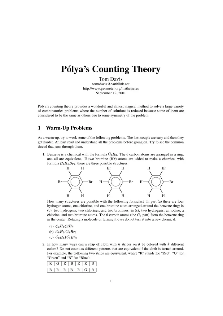
• 1. Benzene is a chemical with the formula

✂✁ ✄☎✁ . The 6 carbon atoms are arranged in a ring,

and all are equivalent. If two bromine ( ✆✞✝ ) atoms are added to make a chemical with formula

✟✁ ✄✞✠ ✆✡✝ ☛ , there are three possible structures: ☞ ☞ ✌ ✌ ☞ ☞ ✌ ✌ ✍✏✎ ✑✏✒

Br H

✌ ✌

H

☞ ☞

Br H

✌ ✌

H

☞ ☞ ☞ ☞ ✌ ✌ ☞ ☞ ✌ ✌ ✍✓✎ ✑✓✒

H Br

✌ ✌

H

☞ ☞

Br H

✌ ✌

H

☞ ☞ ☞ ☞ ✌ ✌ ☞ ☞ ✌ ✌ ✍✓✎ ✑✓✒

H H

✌ ✌

Br

☞ ☞

Br H

✌ ✌

H

☞ ☞

How many structures are possible with the following formulas? In part (a) there are four hydrogen atoms, one chlorine, and one bromine atom arranged around the benzene ring; in (b), two hydrogens, two chlorines, and two bromines; in (c), two hydrogens, an iodine, a chlorine, and two bromine atoms. The 6 carbon atoms (the

✟✁ part) form the benzene ring

in the center. Rotating a molecule or turning it over do not turn it into a new chemical. (a)

✂✁ ✄☎✠ ✞✔ ✆✞✝

(b)

✂✁ ✄ ☛ ✞✔ ☛ ✆✡✝ ☛

(c)

✂✁ ✄ ☛ ✕ ✡✔ ✆✡✝ ☛

• 2. In how many ways can a strip of cloth with

✖

stripes on it be colored with

✗

different colors? Do not count as different patterns that are equivalent if the cloth is turned around. For example, the following two strips are equivalent, where “R” stands for “Red”, “G” for “Green” and “B” for “Blue”: R G R B R R B B R R B R G R 1

SLIDE 2

• 3. In how many ways can a tablecloth that is divided into

✘✚✙✛✘

squares be colored with

✜

colors? There are two answers, depending on whether the tablecloth can be flipped over and rotated or simply rotated to make equivalent patterns.

• 4. In how many ways can a necklace with 12 beads be made with 4 red beads, 3 green beads,

and 5 blue beads? How many necklaces are possible with

✘

beads of

✜ different colors?

• 5. How many ways can you color the corners of a cube such that 3 are colored red, 2 are green,

and 3 are blue?

• 6. How many ways can you color the faces of a dodecahedron with 5 different colors?

2 Illustrative Solutions

We’ll begin with a few problems that are simple enough to solve without P´

• lya’s method, which

we will do, and then we will simply apply the magic method, showing the technique, but without explaining why it works, and we’ll see that the same answer is obtained in both cases.

2.1 A Striped Cloth

✢

In how many ways can a strip of cloth with

✘

stripes on it be colored with

✜

different colors? Do not count as different patterns that are equivalent if the cloth is turned around. For example, the following two strips are equivalent, where “R” stands for “Red”, “G” for “Green” and “B” for “Blue”: R G R B R R B B R R B R G R We will consider a coloring valid if two or more adjacent stripes have the same color. In particular, a solidly-colored strip will be a perfectly good solution (where all the stripes are the same color). If we did not consider strips to be the same when turned around, the answer is obvious—each of the

✘

stripes can be filled with any of

✜

colors, making a grand total of

✜ ✣

possible strips. But this answer is too big, because when you turn the strip around, it matches with one that has the

• pposite coloring. At first it looks like we have double-counted everything, since each strip will

match with its reverse, but this is obviously wrong, if we consider, say, a strip with 2 stripes and three colors. There are

✤ ✥✞✦★✧ colorings (ignoring turning the strip around), but the total number

• f unique colorings given that we are allowed to turn the strip around is obviously not

✧ ✩ ✪ , which

is not an integer. The problem, of course, is that some of the colorings are symmetric (in the case above, 3 of them are symmetric), so the real answer is gotten by adding the number of symmetric cases to the number of non-symmetric cases divided by 2. In this case, the calculation gives:

✤✬✫ ✧✡✭✛✤ ✪ ✦✯✮ ✰

2

SLIDE 3

With this in mind, the general problem is not too hard to solve; we just need to be able to count the symmetric cases. But a symmetric strip has the same stuff on the right as on the left, so once we know what’s on the left, the stuff on the right is determined. There’s a minor problem with odd and even sized strips, but it’s not difficult. For an even number of stripes, say

✱✳✲✵✴ ✶

, there are

✷ ✸

different symmetric possibilities. If

✱

is odd,

✱✛✲✚✴ ✶★✹✛✺ , there are ✷ ✸✂✻✽✼ symmetric possibilities.

Using the floor notation

✾ ✿ ❀ to mean the smallest integer larger than or equal to ✿ , we can write

this in terms of

✷ and ✱

as follows:

✷✽❁ ❂ ❃ ✻❄✼ ❅ ❆ ❇ ❈ ❉

Since this is the number of symmetric colorings, the total number of colorings can be obtained with the following formula:

✷ ❃☎❊ ✷ ❁ ❂ ❃ ✻❄✼ ❅ ❆ ❇ ❈ ✴ ✹✳✷✽❁ ❂ ❃ ✻✽✼ ❅ ❆ ❇ ❈ ✲ ✷ ❃ ✹✳✷ ❁ ❂ ❃ ✻✽✼ ❅ ❆ ❇ ❈ ✴

We can use this formula with

✱✚✲✵❋ and ✷✛✲✵● to solve the original problem, and the answer is

• 135. In addition, check that the following are also true:

❍

If all five slots are green, clearly, there’s only one way to do it.

❍

If the five slots must be filled with three reds and two greens, there are 6 ways to do it.

❍

If you can use two reds, two greens, and a blue, there are 16 ways to color it. Now we will illustrate a method that will solve the problem (and many similar problems besides), but we will not, at first, explain how or why it works. For what appears to be no apparent reason, look at the two permutations of the squares of the strip

• f cloth. Call the colored locations

■ , ❏ , ❑ , ▲ , and ▼ from left to right. There are two symmetry

• perations: leave it alone, or flip it over. In cycle notation, these correspond to:

◆ ■ ❖ ◆ ❏ ❖ ◆ ❑ ❖ ◆ ▲ ❖ ◆ ▼ ❖

and

◆ ■ ▼ ❖ ◆ ❏ ▲ ❖ ◆ ❑ ❖ .

The first one (leave it alone) has 5 1-cycles. The second (flip it over) has 1 1-cycle and 2 2-cycles. Let

P ✼ stand for 1-cycles, P ❇ stand for 2-cycles. In this case there are only 1- and 2-cycles. If there

were 3-cycles, we would use

P ◗ , et cetera.

Indicate the two permutations as follows:

P❙❘ ✼

and

P❄✼ ✼ P❙❇ ❇ . There is one of the first type and one of

the second type, so write the following polynomial which we shall call the “cycle index”:

❚ ✲ ✺✟❯ P❙❘ ✼ ✹✯✺✟❯ P❄✼ ✼ P❙❇ ❇ ✴ ❉

The 2 in the denominator is the total number of permutations and the 1 in front of each term in the numerator indicates that there is exactly one permutation with this structure. Now, do the following strange “substitution”. Since we’re interested in three colors, we’ll substi- tute for

P ✼ the term ◆ ✿❱✹❳❲☎✹✚❨ ❖ and for P ❇ , the term ◆ ✿❙❇✟✹❳❲ ❇✂✹✚❨ ❇ ❖ . We only have P ✼ and P ❇ in

this example, but if there were an

P ❘ , we’d substitute ◆ ✿❙❘✬✹✳❲ ❘✟✹✚❨ ❘ ❖ . Similarly, if there were 4

colors instead of 3, we’d use four unknowns instead of just

✿ , ❲ , and ❨ .

3

SLIDE 4

Doing the substitution, we obtain:

❩★❬✓❭ ❪❴❫❳❵✞❫❳❛ ❜ ❝✂❫✚❭ ❪❴❫❳❵✞❫❳❛ ❜ ❭ ❪❡❞✂❫❳❵ ❞❢❫✳❛ ❞ ❜ ❞ ❣ ❤

(1) which, when expanded, gives:

✐ ❥ ❪✬❵ ❦❙❛✬❫ ✐ ❥ ❪✟❵✂❛ ❦❢❫ ✐ ❧ ❪✟❵ ❞ ❛ ❞ ❫❳❪ ❝ ❫✛❵ ❝ ❫❳❛ ❝ ❫ ✐ ❧ ❪ ❞ ❵ ❞ ❛✡❫ ✐ ❥ ❪ ❦ ❵✟❛✬❫ ✐ ❧ ❪ ❞ ❵✟❛ ❞ ❫❳♠✽❪❡♥❙❵✞❫✳♠✽❪ ♥✽❛✬❫✳♠✽❪✟❵ ♥ ❫❳♠✽❪✡❛ ♥✂❫ ❧ ❪ ❦ ❵ ❞ ❫ ❧ ❪ ❦ ❛ ❞ ❫ ❧ ❪ ❞ ❵ ❦ ❫ ❧ ❪ ❞ ❛ ❦ ❫❳♠✽❵✂❛ ♥✂❫✳♠✽❵ ♥❄❛ ❫ ❧ ❵ ❦ ❛ ❞ ❫ ❧ ❵ ❞ ❛ ❦

Here’s the magic. If you add all the coefficients in front of all the terms:

✐ ❥ ❫ ✐ ❥ ❫ ✐ ❧ ❫❳♦ ♦ ♦ ❫♣♠✂❫ ❧ ❫ ❧ ❬ ✐ ♠ q . And 135 is the total number of colorings! But there’s more. The term ✐ ❧ ❪❡❵ ❞ ❛ ❞ has

a coefficient of 16, and that’s exactly the number of ways of coloring the strip with a blue (

❪ ) two

reds (

❵ ❞ ), and two greens ( ❛ ❞ ). Why on earth does this work?

Actually, there is a much better way to “add all the coefficients”—notice that if we simply sub- stitute 1 for

❪ , ❵ , and ❛ , we get the sum of the coefficients. But there is no need to expand equa-

tion (1) before doing this—just let

❪ ❬ ❵ ❬ ❛ ❬ ✐ in equation (1). This gives us ❭ ♠ ❝❄❫✛♠✂♦ ♠ ❞ ❜ r ❣ ❬ ❭ ❣ s ♠✟❫ ❣ t ❜ r ❣ ❬ ✐ ♠ q .

Depending on how you learn things, you may want to jump ahead to section 3.1 where we look in detail at this simple example of a striped cloth. Alternatively, you can continue reading in order to see a few more examples in detail first before looking at the underlying mathematics.

2.2 Beads on a Necklace

✉

Count the number of ways to arrange beads on a necklace, where there are

✈ different colors

• f beads, and

✇

total beads arranged on the necklace. With a necklace, we can obviously rotate it around, so if we number the beads in order as 1, 2, 3, 4, then for a tiny necklace with only four beads, the pattern “red, red, blue, blue” is clearly the same as “red, blue, blue, red”, et cetera. Also, since the necklace is just made

• f beads, we can turn it over, so if there were four colors, although we cannot rotate “red,

green, yellow, blue” into “blue, yellow, green, red”, we can flip over the necklace and make those two colorings identical. Using standard counting methods, let’s solve this problem in the special case where

✈ ❬ ❣ and ✇ ❬ s

(two colors of beads, and only 4 beads—it’s a very short necklace). Then we will apply P´

• lya’s method and see that it yields the same result.

With 4 beads and two colors, we can just list the possibilities. There is obviously only one way to do it with either all red beads or all blue beads. If there is one red and three blue or the reverse— three reds and one blue, similarly, there’s only one way to do it. If there are two of each, the blue beads can either be together, or can be separated, so there are two ways to do it. In total, there are thus 6 solutions. Now let’s try P´

• lya’s method:

4

SLIDE 5

If the bead positions are called

① , ② , ③ , and ④ , here are the permutations that map the necklace into

itself:

⑤ ① ⑥ ⑤ ② ⑥ ⑤ ③ ⑥ ⑤ ④ ⑥ , ⑤ ① ④ ③ ② ⑥ , ⑤ ① ③ ⑥ ⑤ ② ④ ⑥ , ⑤ ① ② ③ ④ ⑥ , ⑤ ① ④ ⑥ ⑤ ② ③ ⑥ , ⑤ ① ③ ⑥ ⑤ ② ⑥ ⑤ ④ ⑥ , ⑤ ① ② ⑥ ⑤ ③ ④ ⑥ , and ⑤ ② ④ ⑥ ⑤ ① ⑥ ⑤ ③ ⑥ . (Check

these.) Note that we are listing even the 1-cycles (the beads that don’t move) because it will help us in setting up the equation. In the notation we used previously, we can write down the cycle index:

⑦⑨⑧✓⑩ ❶❡❷ ❸✡❹❳❺ ❶❙❻ ❸ ❶ ❻ ❹✳❼ ❶❙❻ ❻ ❹✳❺ ❶ ❷ ❽ ❾

Since there are three permutations having 2 2-cycles, there is a

❼ in front of the term ❶❙❻ ❻ , et cetera.

Let

❶ ❸ ⑧ ⑤ ❿ ❹❳➀ ⑥ , ❶ ❻ ⑧ ⑤ ❿ ❻ ❹❳➀ ❻ ⑥ , and ❶ ❷ ⑧ ⑤ ❿ ❷ ❹❳➀ ❷ ⑥ . Since there are only two colors, we only

need

❿

and

➀ . Substitute as before to obtain: ⑦⑨⑧ ⑤ ❿ ❹❳➀ ⑥ ❷ ❹❳❺ ⑤ ❿ ❹❳➀ ⑥ ❻ ⑤ ❿ ❻ ❹✛➀ ❻ ⑥ ❹✳❼ ⑤ ❿ ❻ ❹❳➀ ❻ ⑥ ❻ ❹✳❺ ⑤ ❿ ❷ ❹❳➀ ❷ ⑥ ❽ ❾

(2) If we expand, we obtain:

❿ ❷ ❹ ❿❙➁ ➀✞❹❳❺ ❿ ❻ ➀ ❻ ❹ ❿ ➀ ➁ ❹✛➀ ❷ ❾

It’s easy to check that these terms correspond to the 6 ways beads could be arranged, where there’s a unique way to do it unless there are two of each color, in which case there are two arrangements. Also notice that it gives our detailed count as well. If we think of the

❿

as corresponding to a “red” bead, and

➀ to a “blue” bead, the coefficient in front of the term ❿ ❷ (which is 1) corresponds to the

number of ways of making a necklace with four red beads. The 2 in front of the

❿ ❻ ➀ ❻ term means

that there are two necklaces with two beads of each color, et cetera. And notice again that by substituting

❿ ⑧ ➀ ⑧ ⑩ into equation (2) we obtain the total count: ❺ ❷ ❹✳❺✡➂ ❺ ❻ ➂ ❺✬❹❳❼✡➂ ❺ ❻ ❹❳❺✡➂ ❺ ❽ ⑧✓⑩ ➃ ❹ ⑩ ➃ ❹ ⑩ ❺✬❹❳➄ ❽ ⑧ ➃ ❾

Now let’s try something slightly more interesting. What if there are three colors? Let’s call the colors “R”, “G” and “B”, for “red”, “green”, and “blue”. Here’s a brute-force count. Check to see that you agree with the counts below:

➅

All the same color (3 ways)

➅

Three of one color and one of another (6 ways)

➅

Two of one color and two of another (3 ways)

➅

Two of one color and two different colors (3 ways) In the previous example (4 beads and 2 colors) we worked out how many ways there were to do all but the last one—one way with all the same color or with 3 of one color, and two ways with two of each of two colors. A little bit of scratch work should convince you that there are also only two ways to do the last case (the two beads of the same color can be adjacent or not). 5

SLIDE 6

Thus the grand number of ways to place beads of 3 different colors on a necklace with 4 beads is:

➆✡➇ ➈✂➉✳➊✡➇ ➈✂➉✳➆✡➇ ➋✬➉❳➆✡➇ ➋✞➌✯➋ ➈ ➍

With three beads, the equation for the cycle index

➎

(corresponding to equation (2) above) is:

➎ ➌ ➏ ➐ ➉❳➑✞➉✳➒ ➓ ➔✟➉❳➋ ➏ ➐ ➉❳➑✞➉❳➒ ➓ → ➏ ➐ →✟➉✛➑ →✂➉❳➒ → ➓ ➉✡➆ ➏ ➐ →✂➉❳➑ →❢➉✳➒ → ➓ →✂➉❳➋ ➏ ➐ ➔✟➉✛➑ ➔✟➉❳➒ ➔ ➓ ➣ ➍

(3) If we just want the grand total, we can substitute

➐ ➌✚➑❴➌✯➒✞➌⑨➈ into equation (3) to obtain: ➆ ➔ ➉❳➋✡➇ ➆ → ➇ ➆✬➉❳➆✡➇ ➆ → ➉✳➋✡➇ ➆ ➣ ➌ ➣ ➈❢➉✳↔ ↕✡➉❳➋ ➙✟➉❳➊ ➣ ➌ ➈ ➊ ➣ ➣ ➌✯➋ ➈ ➍

We can, of course, expand equation (3) and obtain:

➏ ➐ ➔✬➉✛➑ ➔✟➉❳➒ ➔ ➓❄➉ ➏ ➐❡➛ ➑☎➉ ➐❙➛ ➒✡➉ ➐ ➑ ➛ ➉ ➐ ➒ ➛ ➉✛➑ ➛ ➒✬➉❳➑ ➒ ➛ ➓ ➉ ➏ ➋ ➐ → ➑ →✂➉✳➋ ➐ → ➒ →✂➉❳➋ ➑ → ➒ → ➓✽➉ ➏ ➋ ➐ → ➑ ➒✡➉❳➋ ➐ ➑ ➒ →❢➉✳➋ ➐ ➑ → ➒ ➓ ➍

Note that groups corresponding to the various combinations of beads in the list above are gathered together with parentheses. Clearly with a small numbers of beads and colors, it’s probably easier just to do a brute-force enumeration, but if the number of beads or colors gets large, P´

• lya’s method becomes more and

more attractive. To illustrate, look at a necklace with 17 beads in it. A little playing around will show you that the cycle index polynomial you need is this:

➎ ➌➝➜❄➞ ➟ ➞ ➉✚➈ ➊ ➜ ➞ ➟ ➉✚➈ ➙ ➜ ➞ ➜❙➠ → ➆ ↕ ➍

Let’s try to solve this with 4 colors of beads to obtain:

➎ ➌ ➏ ➡ ➉ ➐ ➉✛➑☎➉❳➒ ➓ ➞ ➟ ➉✚➈ ➊ ➏ ➡ ➞ ➟ ➉ ➐ ➞ ➟ ➉✛➑ ➞ ➟ ➉✳➒ ➞ ➟ ➓ ➉✞➈ ➙ ➏ ➡ ➉ ➐ ➉❳➑✞➉❳➒ ➓ ➏ ➡ →✟➉ ➐ →✂➉✛➑ →✂➉❳➒ → ➓ ➠ ➆ ↕ ➍

(4) Substituting

➡ ➌ ➐ ➌✏➑✯➌✓➒✳➌➢➈ into this yields ↔ ➤ ↔ ↕ ➋ ➈ ➆ ↕ ↕

• solutions. If you have a really

strong stomach, you can multiply out the expression for

➎

and get the breakdown for various color combinations. Notice that if you have a particular problem, you can often solve it without a complete expansion

• f the expression for

➎ . For example, if you want to know, for the 17-bead necklace, how many

examples there are with 2 red, 4 blue, 3 yellow, and 8 green beads, all you need to do is to calculate the coefficient of

➡ → ➐ ➔ ➑ ➛ ➒ ➠ and you will have the number you want. A very valuable

tool is the formula for multinomial coefficients (which is just a generalization of the formula for binomial coefficients). Here is the multinomial expansion of

➏ ➐ ➉✚➑ ➓ ➥ , of ➏ ➐ ➉✳➑❴➉✯➒ ➓ ➥

and of

➏ ➡ ➉ ➐ ➉➦➑✂➉♣➒ ➓ ➥ . It’s easy to see what the generalization to any number of variables will be. (The

6

SLIDE 7

binomial expansion has been written in a slightly different form than usual so you can see how it relates to the more complicated versions.)

➧ ➨❱➩✛➫ ➭ ➯➳➲➸➵ ➺ ➻ ➼ ➽ ➾ ➺ ➚ ➼ ➪ ➶ ➹❢➘ ➴ ➘ ➷❡➘ ➨❙➬ ➫ ➮✬➲ ➯ ➵ ➬ ➱❡✃ ➹❢➘ ➴ ➘ ➧ ➹➦❐ ➴ ➭ ➘ ➨❡➬ ➫ ➯ ❒❙➬ ➧ ➨❴➩✛➫✞➩✳❮ ➭ ➯➳➲❰➵ ➺ ➻ ➼ ➻ Ï ➽ ➾ ➺ ➚ ➼ ➚ Ï ➪ ➶ ➹❢➘ ➴ ➘ ➷ ➘ Ð❙➘ ➨❡➬ ➫ ➮ ❮ Ñ ➧ Ò✚➩❳➨❴➩✛➫✞➩✳❮ ➭ ➯➳➲ ➵ ➺ ➻ ➼ ➻ Ï ➻ Ó ➽ ➾ ➺ ➚ ➼ ➚ Ï ➚ Ó ➪ ➶ ➹❢➘ ➴ ➘ ➷ ➘ Ð❙➘ Ô ➘ Ò✬➬ ➨ ➮ ➫ Ñ ❮ Õ Ö

To illustrate with our example above to count the number of necklaces with 2 red, 4 blue, 3 yellow, and 8 green beads, we look at the three terms in the numerator of equation (4). We are looking for coefficients of terms like this:

Ò✬× ➨❡Ø ➫ Ù ❮ Ú .

In

➧ Ò★➩✳➨❱➩✳➫☎➩✚❮ ➭ Û Ü , the coefficient will be Ý Þ ➘ ß ➧ à ➘ á❡➘ â ➘ ã ➘ ➭ . There will be no appropriate terms

from the expansion of

Ý ä ➧ Ò✞Û Ü❄➩➦➨❄Û Ü✽➩➦➫❡Û Ü❄➩♣❮ Û Ü ➭ . From Ý Þ ➧ Ò✛➩➦➨✡➩➦➫✟➩♣❮ ➭ ➧ Ò✬×❄➩➦➨❙×❄➩➦➫ ×❄➩♣❮ × ➭ Ú ,

the part on the right will only generate even powers of the variables, so the only way to get the term we want is to pick

➫

from the first term, and

Ò✡× ➨ Ø ➫ × ❮ Ú from the second, and this will occur ã ➘ ß ➧ Ý ➘ à ➘ Ý ➘ á❡➘ ➭ times. So the coefficient we are interested in is: Ý Þ ➘ à ➘ á❡➘ â ➘ ã ➘ ➩ Ý Þ ã ➘ Ý ➘ à ➘ Ý ➘ á❡➘ â á ➲✯å æ Ý â à æ Ö

Thus, there are 901320 ways to make such a necklace.

3 What’s Going On?

The construction of the functions above is rather mysterious, so let’s spend a little time looking at why it might work. We’ll begin by examining some very simple cases of symmetry to see why P´

• lya’s method works on these.

Note that none of the sections below provides a proof that the method works; each section simply provides another way to think about what is going on.

3.1 Striped Cloth Analysis

Let’s examine the first problem we looked at again, where we counted colorings of a striped cloth, but we’ll start from the simplest possible example—a piece of cloth with one stripe. Clearly, if there are

➹

colors available, there are

➹

ways to color the stripe. There is only one permutation:

➧ Ý ➭ , so the associated equation for ➹

colors will look like this:

ç ➲➝è Û Û Ý ➲ ➨ Û ➩✛➨ × ➩✯é é é ➩❳➨ ➯ Ý Ö

This has the

➹

terms

➨ Û , ➨ × , ... ➨ ➯ .

7

SLIDE 8

But perhaps that is too simple; let’s consider a cloth with two strips. If the colors are called

ê✞ë ì❱ë í✡ë î î î , then here are the possibilities for ï ë ð ë ñ ë and ò

colors, where

ó ê✬í✡ô , for example,

represents the cloth with one stripe colored

ê

and the other colored

í . Of course ó ê✬í✬ô is the same

as

ó í✞ê✟ô : ï✡õöó ê✬ê✟ô ÷

(5)

ð õöó ê✬ê✟ô ó ì✞ì✞ô ÷ ó ê✬ì✞ô

(6)

ñ õöó ê✬ê✟ô ó ì✞ì✞ô ó í✡í✡ô ÷ ó ê✬ì✞ô ó ê✬í✬ô ó ì☎í✬ô

(7)

ò❴õöó ê✬ê✟ô ó ì✞ì✞ô ó í✡í✡ô ó ø❴ø ô ÷ ó ê✬ì✞ô ó ê✬í✬ô ó ê ø ô ó ì✞í✡ô ó ì ø ô ó í ø ô

(8) Notice that if there are

ù

colors, there will be

ú û ü ý strips of the form ó ê✬ì✞ô , where ê

and

ì

are different colors and

ù

• f the form

ó ê✬ê✟ô . Thus the total number of colorings is ú û ü ý✟þ✛ù .

Going back to the formulation in terms of permutations, there are only two of them:

ÿ

• ✁

ÿ ✂ ✁ and ÿ

• ✂

✁ . The formula for ✄

is:

✄✆☎ ✝ ü ✞ þ ✝ ü ð✠✟

Doing the magic substitution for

ù

colors gives:

✄✡☎ ÿ ☛ ✞ þ☞☛ ü þ î î î þ☞☛ û ✁ ü þ✚ÿ ☛ ü ✞ þ✌☛ ü ü þ î î î þ✌☛ ü û ✁ ð

(9)

☎ ÿ ☛ ü ✞ þ☞☛ ü ü þ î î î þ☞☛ ü û ✁ þ✎✍ ✞ ✏✒✑ ✓✕✔ ✏ û ☛ ✑ ☛ ✔ ✟

(10) There are

ú û ü ý terms of the form ☛ ✑ ☛ ✔ and ù

terms of the form

☛ ü ✑ (which you can think of as ☛ ✑ ☛ ✑

for the benefit of a comparison to the lists in (5) through (8), above). Every symmetry of the strip reduces the number of possible patterns. The inclusion of the permu- tation

ÿ

• ✂

✁ makes patterns ó ê✬ì✡ô and ó ì✞ê✟ô equivalent, where they would be considered different

without that symmetry. Consider what happens to the equation for

✄

as additional symmetries are added (and the number

• f distinct colorings decreases). The denominator of

✄

is increased by 1 for each new permuta- tion and although new terms are added to the numerator, there are fewer of them. Consider the difference between the two terms in the numerator for

✄

in equation (9)—the first expression,

ÿ ☛ ✞ þ î î î þ✖☛ û ✁ ü makes ù ü terms (counting multiplicity). The second expression, ÿ ☛ ü ✞ þ î î î þ✗☛ ü û ✁ ,

• nly adds

ù

terms. In fact, the more things a permutation moves around, the fewer terms it generates in the numerator. Let’s count the terms for all the possible shapes of permutations of 4 items with

ù

colors: Count Shape Formula Terms 1

ÿ

• ✁

ÿ ✂ ✁ ÿ ✘ ✁ ÿ ✙ ✁ ✝✕✚ ✞ ù ✚

6

ÿ

• ✂

✁ ÿ ✘ ✁ ÿ ✙ ✁ ✝ ü ✞ ✝ ü ù✜✛

3

ÿ

• ✂

✁ ÿ ✘ ✙ ✁ ✝ ü ü ù ü

8

ÿ

• ✂

✘ ✁ ÿ ✙ ✁ ✝ ✞ ✝ ✛ ù ü

6

ÿ

• ✂

✘ ✙ ✁ ✝ ✚ ù

8

SLIDE 9

The count is the number of permutations having that shape; the formula is what goes in the numer- ator of

✢ , and the number of terms is counted with multiplicity—in other words, ✣✜✤ ✣✕✥ is counted

differently from

✣✕✥ ✣✜✤ . Thus the permutation that doesn’t collapse any colorings, ✦ ✧ ★ ✦ ✩ ★ ✦ ✪ ★ ✦ ✫ ★ ,

adds the most terms to the numerator,

✬✒✭ . The permutation that moves every color position to

another,

✦ ✧ ✩ ✪ ✫ ★ , has the fewest, ✬ . Even though ✦ ✧ ✩ ★ ✦ ✪ ✫ ★ moves everything, it moves them in a

restricted way—the colors in slots

✧

and

✩ cannot mix into slots ✪ and ✫

under this permutation, and hence, since it does less collapsing, it adds more to the numerator of

✢

(

✬ ✥ terms).

3.2 A Fixed Point

As a second example, let’s consider a situation where the allowable symmetries always leave one region fixed. In the example of the strip of cloth that we considered in section (2.1), if there are an odd number of stripes, the center stripe is fixed—it always goes to itself under any symmetry

• peration. Here’s another example: imagine a structure built with tinker-toys with a central hub

and eight hubs extending from it on sticks, as in figure 1. If you’ve got

✬

different colors of hubs and you want to count the number of configurations that can be made, it’s pretty clear that the central hub will always go to itself in any symmetry operation. It’s quite easy to make up any number of additional examples. Figure 1: Tinkertoy Object In any example where one of the positions to be colored is fixed by all of the symmetry operations, it’s clear that if you can count the number of configurations of the rest of the object when

✬

colors are used, to get the grand total when the additional fixed position is included, you’ll simply multiply your previous total by

✬ . What does this mean in terms of the permutations and the

polynomial that we construct? If you have the polynomial corresponding to the figure without the fixed point, to include the fixed point, you simply need to add a 1-cycle to each of those you already have. For example, suppose your figure consists of a triangle with the point at the center as well that is fixed. If the three vertices of the triangle are called

✧ , ✩ , and ✪ , and the point at the center is called ✫ , without the

central point here are the permutations:

✦ ✧ ★ ✦ ✩ ★ ✦ ✪ ★ ✮ ✦ ✧ ✩ ★ ✦ ✪ ★ ✮ ✦ ✧ ✪ ★ ✦ ✩ ★ ✮ ✦ ✩ ✪ ★ ✦ ✧ ★ ✮ ✦ ✧ ✩ ✪ ★ ✮ ✦ ✧ ✪ ✩ ★ ✯

With point

✫ included, here they are: ✦ ✧ ★ ✦ ✩ ★ ✦ ✪ ★ ✦ ✫ ★ ✮ ✦ ✧ ✩ ★ ✦ ✪ ★ ✦ ✫ ★ ✮ ✦ ✧ ✪ ★ ✦ ✩ ★ ✦ ✫ ★ ✮ ✦ ✩ ✪ ★ ✦ ✧ ★ ✦ ✫ ★ ✮ ✦ ✧ ✩ ✪ ★ ✦ ✫ ★ ✮ ✦ ✧ ✪ ✩ ★ ✦ ✫ ★ ✯

The new polynomial will simply have another

✰ ✤ in every term, so it can be factored out, and the

new polynomial will simply have an additional factor of

✦ ✣✜✤✒✱✖✣✕✥✜✱✖✣✒✲✒✱✌✳ ✳ ✳ ✱✖✣✕✴ ★ (assuming you

9

SLIDE 10

are working the problem with

✵

• colors. The total count will thus simply be

✵

times the previous count, as we noted above. To make this concrete, look at this triangle case with three colors. Ignoring point

✶ , we have: ✷✹✸✻✺✒✼ ✽✿✾✌❀ ✺ ✽ ✺ ❁ ✾❃❂ ✺ ✼ ❄ ❅

If we include

✶ , we get: ✷✆✸ ✺✕❆ ✽ ✾❃❀ ✺ ❁ ✽ ✺ ❁ ✾❃❂ ✺ ✽ ✺ ✼ ❄ ✸ ✺ ✽ ❇ ✺✒✼ ✽ ✾❃❀ ✺ ✽ ✺ ❁ ✾✌❂ ✺ ✼ ❈ ❄ ❅

If we substitute

❇ ❉ ✾✌❊❋✾✌● ❈ in the usual way, we obtain: ✷✆✸ ❉ ✼ ✾✌❊ ✼ ✾❃● ✼ ✾ ❉ ❁ ❊❋✾ ❉ ❁

• ❍✾

❉ ❊ ❁ ✾ ❉

• ❁

✾✌❊ ❁

• ✿✾☞❊
• ❁

✾ ❉ ❊

• ■

and for

✷✿❏ we obtain: ✷ ❏ ✸ ❇ ❉ ✾✌❊❋✾✌● ❈ ✷ ✸ ❇ ❉ ✾✌❊❋✾✌● ❈ ❇ ❉ ✼ ✾✌❊ ✼ ✾❃● ✼ ✾ ❉ ❁ ❊❋✾ ❉ ❁

• ❍✾

❉ ❊ ❁ ✾ ❉

• ❁

✾✌❊ ❁

• ✿✾☞❊
• ❁

✾ ❉ ❊

• ❈

❅

3.3 Independent Parts

Assume that the allowable symmetries are, in a sense, disconnected. As a simple example, imagine a child’s rattle toy that has hollow balls on both ends of a handle, and one of the balls contains 3 marbles while the other contains two. In how many ways can this rattle be filled with marbles of 4 different colors? Or perhaps a more practical example is this example from chemistry: Imagine a carbon atom hooked to a nitrogen atom. You can connect three other atoms to the carbon and two

• ther atoms to the nitrogen. If the other atoms to be hooked on are chosen from among hydrogen,

fluorine, chlorine, and iodine, how many different types of chemicals are possible1? In the rattle example, there is no ordering to the three marbles on one end of the rattle and to the two on the other end, but the two ends cannot be swapped since they contain different numbers of

• marbles. All the symmetries involve swapping among the three or among the two. So if

❑ , ▲ , and ▼ represent the marbles on the three side, and if ✶ and ◆ represent those on the two side, we can

take what’s called mathematically a “direct product” of the individual groups to get the symmetry group for the entire rattle. All the entries in the table below form the symmetry group for the rattle as a whole. Each is composed of a product of one symmetry from the three side and one from the two side:

❖ P ◗ ❖ ❘ ◗ ❖ ❙ ◗❚❖ P ◗ ❖ ❘ ❙ ◗❚❖ P ❘ ◗ ❖ ❙ ◗❚❖ P ❙ ◗ ❖ ❘ ◗❚❖ P ❘ ❙ ◗❚❖ P ❙ ❘ ◗ ❖ ❯ ◗ ❖ ❱ ◗ ❖ P ◗ ❖ ❘ ◗ ❖ ❙ ◗ ❖ ❯ ◗ ❖ ❱ ◗❲❖ P ◗ ❖ ❘ ❙ ◗ ❖ ❯ ◗ ❖ ❱ ◗❲❖ P ❘ ◗ ❖ ❙ ◗ ❖ ❯ ◗ ❖ ❱ ◗❲❖ P ❙ ◗ ❖ ❘ ◗ ❖ ❯ ◗ ❖ ❱ ◗❲❖ P ❘ ❙ ◗ ❖ ❯ ◗ ❖ ❱ ◗❲❖ P ❙ ❘ ◗ ❖ ❯ ◗ ❖ ❱ ◗ ❖ ❯ ❱ ◗ ❖ P ◗ ❖ ❘ ◗ ❖ ❙ ◗ ❖ ❯ ❱ ◗❳❖ P ◗ ❖ ❘ ❙ ◗ ❖ ❯ ❱ ◗❳❖ P ❘ ◗ ❖ ❙ ◗ ❖ ❯ ❱ ◗❳❖ P ❙ ◗ ❖ ❘ ◗ ❖ ❯ ❱ ◗❳❖ P ❘ ❙ ◗ ❖ ❯ ❱ ◗❳❖ P ❙ ❘ ◗ ❖ ❯ ❱ ◗

Thus, when we have a term like

✺ ✽ ✺ ❁ from the three group and an element like ✺ ❁ ✽

in the two group, the combination will simply generate a term that is the product of the two:

✺✒✼ ✽ ✺ ❁ , and this

1Although it may seem that these two examples are identical, they are not—the marbles in the three side can be swapped

in any way (so there are 6 symmetries); on the carbon atom, they can only be rotated (so there are only 3 symmetries).

10

SLIDE 11

will happen in every case. It should be easy to see (if you don’t see it, work out the polynomials and check) that if

❨✜❩ is the cycle index polynomial for the two group and ❨✜❬ is the one for the three

group, then the cycle index polynomial for the entire permutation group will simply be

❨✜❩ ❨✜❬ , and

it’s clear that the counts of possible configurations will simply be the products of the individual configurations.

3.4 Cyclic Permutations

Next, let’s look at one example that is still simple, but a bit more complicated than what we’ve examined up to now—we’ll examine the case where the positions can be rotated by any amount, but cannot be flipped over. For concreteness, assume that you’ve got a circular table, and you wish to set the table with plates of

❭

different colors, but rotations of the plates around the table are considered to be equivalent. In how many different ways can this be done? It seems that cyclic permutations are pretty simple, but as you’ll see, at least a little care must be

• taken. We’ll examine two examples that seem similar at first, but illustrate most of the interesting

behavior that you can see. We’ll look at the groups of cyclic permutations of both 6 and 7 elements. Call the positions

❪ , ❫ , ❴ , ❵ , ❛ , and ❜

(for the table with 6 place settings), and we’ll add position

❝

for the table with seven. Listed below are the complete sets of cyclic permutations of 6 or 7

• bjects.

❪❞❫✡❴❡❵✡❛❢❜ ❣ ❪ ❤ ❣ ❫ ❤ ❣ ❴ ❤ ❣ ❵ ❤ ❣ ❛ ❤ ❣ ❜✒❤ ❪❞❫✡❴❡❵✡❛❢❜ ❣ ❪ ❫ ❴ ❵ ❛ ❜✒❤ ❫✐❴❡❵❞❛❢❜❞❪ ❣ ❪ ❴ ❛ ❤ ❣ ❫ ❵ ❜✒❤ ❴❢❵❞❛❢❜❞❪❥❫ ❣ ❪ ❵ ❤ ❣ ❫ ❛ ❤ ❣ ❴ ❜✒❤ ❵✡❛❢❜❞❪❥❫✡❴ ❣ ❪ ❛ ❴ ❤ ❣ ❫ ❜✒❵ ❤ ❛❢❜❞❪❞❫✡❴❡❵ ❣ ❪ ❜✒❛ ❵ ❴ ❫ ❤ ❜❞❪❥❫✐❴❡❵❞❛ ❪❥❫✐❴❡❵❞❛❢❜ ❝ ❣ ❪ ❤ ❣ ❫ ❤ ❣ ❴ ❤ ❣ ❵ ❤ ❣ ❛ ❤ ❣ ❜✒❤ ❣ ❝ ❤ ❪❥❫✐❴❡❵❞❛❢❜ ❝ ❣ ❪ ❫ ❴ ❵ ❛ ❜ ❝ ❤ ❫✡❴❢❵❞❛❢❜ ❝ ❪ ❣ ❪ ❴ ❛ ❝ ❫ ❵ ❜✒❤ ❴❡❵❞❛❦❜ ❝ ❪❥❫ ❣ ❪ ❵ ❝ ❴ ❜✒❫ ❛ ❤ ❵❞❛❢❜ ❝ ❪❥❫✡❴ ❣ ❪ ❛ ❫ ❜✒❴ ❝ ❵ ❤ ❛❢❜ ❝ ❪❥❫✐❴❡❵ ❣ ❪ ❜✒❵ ❫ ❝ ❛ ❴ ❤ ❜ ❝ ❪❥❫✐❴❡❵❞❛ ❣ ❪ ❝ ❜✒❛ ❵ ❴ ❫ ❤ ❝ ❪❞❫✡❴❡❵✡❛❢❜

Notice that the lower table (for 7 elements) has every permutation except for the identity the same (in terms of cycle structure), while the table with 6 elements has a variety of cycle structures. The reason, of course, is that 7 is a prime number. With the 6-element example, three rotations

• f two positions or two rotations of three positions bring you back to where you started. If the

plates on the 6-table are colored “red, green, red, green, red, green”, they rotate to themselves after every rotation of 2 positions, or if the coloring is “red, green, blue, red, green, blue” they rotate to themselves after a rotation of three positions. In fact, it’s easy to see that something similar will happen for any integer multiples of the table size. If the table, however, has a prime number of positions, the only way to bring it back to the initial configuration is to leave it alone, or turn it through an entire

❧ ♠ ♥ ♦ rotation.

11

SLIDE 12

Thus if we are counting colorings that are unique even taking rotations into account, we should expect different behavior if the number of positions is prime or not. Clearly the cycle indices of the two examples above look quite different:

♣rq❍s✻t q ✉✿✈ t✒✇ ①②✈✌③ t ① ✇ ✈✌③ t q ④ ⑤

and

♣✜⑥✿s⑦t ⑥ ✉✿✈ ④ t ⑥ ⑧⑩⑨

3.5 Three More Examples

Now let’s look at three related examples in detail to see exactly how the cycle structure of the symmetry permutations affect the number of possible colorings. We will look at coloring the three points of a triangle, but with three different interpretations. We will call the three vertices of the triangle that can be colored

❶ , ❷ , and ❸ :

• 1. No symmetry operations are allowed. In other words, coloring

❶

red and

❷ and ❸ green is

different from coloring

❷ red and ❶

and

❸ green. The only symmetry operation allowed is

to leave it unchanged. The symmetry group is this:

❹ ❺ ❶ ❻ ❺ ❷ ❻ ❺ ❸ ❻ ❼ . The cycle index is this: ♣ ✉ s ❺ t✒✇ ✉ ❻ ❽ ❾ .

• 2. Rotating the triangle (but not flipping it over) is allowed, So the triangle can be rotated to

three different positions, or three different symmetry operations. The symmetry group is this:

❹ ❺ ❶ ❻ ❺ ❷ ❻ ❺ ❸ ❻ ⑤ ❺ ❶ ❷ ❸ ❻ ⑤ ❺ ❶ ❸ ❷ ❻ ❼ . The cycle index is this: ♣ ✇ s ❺ t✒✇ ✉✿✈❃③ t ✇ ❻ ❽ ❿ .

• 3. Rotating and flipping the triangle is allowed. In this case, there are 6 symmetry operations.

The symmetry group is this:

❹ ❺ ❶ ❻ ❺ ❷ ❻ ❺ ❸ ❻ ⑤ ❺ ❶ ❷ ❸ ❻ ⑤ ❺ ❶ ❸ ❷ ❻ ⑤ ❺ ❶ ❻ ❺ ❷ ❸ ❻ ⑤ ❺ ❷ ❻ ❺ ❶ ❸ ❻ ⑤ ❺ ❸ ❻ ❺ ❶ ❷ ❻ ❼ . The cycle

index is this:

♣✜q✿s ❺ t✒✇ ✉✿✈ ❿ t ✉ t ① ✈✌③ t ✇ ❻ ❽ ④ .

In each case, let’s consider the situation with three different colors allowed, so we’ll be plugging in

❺ ➀✒➁ ✈✌➂ ➁ ✈✌➃ ➁ ❻ for t ➁ in the cycle indices above. Here’s what happens in the three cases above:

• 1. First of all, it’s clear in this case that every different assignment of colors leads to a unique

coloring since only the identity symmetry operation is allowed. Thus there should be

❿ ✇ s ③ ⑧ colorings. It’s probably easiest to see what’s going on by expanding ♣ ✉ s ❺ ➀ ✈✌➂❋✈❃➃ ❻ ✇

at first without using the commutative law to condense the possibilities:

♣ ✉ s ➀ ➀✕➀ ✈ ➀ ➀ ➂❋✈ ➀ ➀ ➃✿✈ ➀ ➂ ➀ ✈ ➀ ➂ ➂❋✈ ➀ ➂ ➃❍✈ ➀ ➃ ➀ ✈ ➀ ➃ ➂❋✈ ➀ ➃ ➃✿✈ ➂ ➀ ➀ ✈✌➂ ➀ ➂❋✈✌➂ ➀ ➃✿✈☞➂ ➂ ➀ ✈✌➂ ➂ ➂✿✈✌➂ ➂ ➃❍✈☞➂ ➃ ➀ ✈✌➂ ➃ ➂❋✈☞➂ ➃ ➃❍✈ ➃ ➀✕➀ ✈✌➃ ➀ ➂❋✈❃➃ ➀ ➃❍✈✌➃ ➂ ➀ ✈❃➃ ➂ ➂❋✈✌➃ ➂ ➃❍✈✌➃ ➃ ➀ ✈❃➃ ➃ ➂✿✈❃➃ ➃ ➃ s ➀ ✇ ✈✌➂ ✇ ✈✌➃ ✇ ✈ ❿ ❺ ➀ ① ➂❋✈ ➀ ① ➃❍✈ ➀ ➂ ① ✈ ➀ ➃ ① ✈✌➂ ① ➃✿✈☞➂ ➃ ① ❻ ✈ ④ ➀ ➂ ➃

Before grouping like elements, the 27 terms correspond exactly to the 27 colorings, where

➀ ➂ ➂ corresponds to color ➀

in slot

❶ , ➂ in slot ❷ , and ➂ in slot ❸ , et cetera.

After grouping, the fact that there are 3 terms like

➀ ① ➃ means that there are 3 ways to color

using two

➀ s and a ➂ .

There’s only one symmetry operation (the identity), so we only divide by 1. 12

SLIDE 13

• 2. In this case, since rotations can make certain colorings identical we’ll expect to have fewer

final configurations. Think of it as making all 27 colorings as in the first example, and then grouping together those that are the same.

➄✜➅❍➆✻➇ ➅ ➈✿➉✌➊ ➇ ➅ ➋➍➌

so we’re adding a bunch of terms to the numerator with the

➊ ➇ ➅ , but we are also dividing by

3 instead of by 1. Notice that the expansion of

➇ ➅ ➈

has more terms than any of the other possibilities—

➊ ➇ ➅

in this case, and an additional

➋ ➇ ➈ ➇ ➎ in the following example. In this case, the ➊ ➇ ➅ will

contribute

➊ ➏ ➐ ➅ ➉❍➑ ➅ ➉✿➒ ➅ ➓

—just six terms (counting each one twice because of the coefficient

• f 2). So there are now

➊ ➔r➉➣→ ➆ ➋ ➋ terms in the numerator, but we divide by 3 making only

11 final terms:

➄✜➅✿➆ ➐ ➅ ➉✌➑ ➅ ➉❃➒ ➅ ➉↔➏ ➐ ➎ ➑❋➉☞➐ ➎ ➒❍➉✌➐ ➑ ➎ ➉☞➐✒➒ ➎ ➉✌➑ ➎ ➒❍➉✌➑ ➒ ➎ ➓ ➉✌➊ ➐✕➑ ➒ ↕

There are 2

➐✕➑ ➒

terms since three different colors can be arranged clockwise or counter- clockwise, and since the triangle cannot be flipped over, these are distinct.

• 3. In this case with all possible rearrangements allowed, there should be even fewer examples

(in this small case, it will only be reduced by 1, since we only will combine the two

➐✕➑ ➒

terms). But let’s look at the cycle index. The numerator will be the same as in the example above, but with the addition of the term

➋ ➇ ➈ ➇ ➎ . The denominator will be doubled to 6.

For three colors,

➋ ➇ ➈ ➇ ➎ ➆ ➋ ➏ ➐✖➉❃➑➙➉➛➒ ➓ ➏ ➐ ➎ ➉❃➑ ➎ ➉↔➒ ➎ ➓

, which will have 27 terms (again counting multiplicity). So combining this with the 33 terms we’ve already considered, we have

➏ ➋ ➋ ➉✌➊ ➔ ➓ ➜ → ➆✆➝ ➞ terms: ➄r➟❍➆ ➐ ➅ ➉✌➑ ➅ ➉✌➒ ➅ ➉➛➏ ➐ ➎ ➑❋➉✌➐ ➎ ➒❍➉✌➐ ➑ ➎ ➉✌➐✕➒ ➎ ➉☞➑ ➎ ➒✿➉☞➑ ➒ ➎ ➓ ➉✌➐ ➑ ➒✕↕

It’s a good idea to examine these cases yourself a bit more carefully to see exactly how the terms combine to reduce the number of colorings. You should also try to construct some other cases. For example, again with the same triangle as above, suppose the only symmetry operation allowed is to leave

➠ in place and to swap ➡ and ➢ . Try it with 2 colors, or 4 colors. Try a square with various

symmetry operations, et cetera.

3.6 Yet Another Approach

Let us again consider the simple case of an object that has three slots to be colored, and we will consider various symmetry operations on it and what each would do to the count of the total colorings. 3.6.1 Only the Identity As we’ve said before, if no symmetry operations are allowed, there is only one symmetry oper- ation, the identity:

➏ ➠ ➓ ➏ ➡ ➓ ➏ ➢ ➓

, yielding

➤ ➅

colorings, where

➤

is the number of available colors.

➄✆➆ ➇ ➅ ➈ ➆ ➏ ➐ ➈ ➉↔➥ ➥ ➥ ➉✌➐✕➦ ➓ ➅

has

➤ ➅

terms so everything works out in an obvious way. 13

SLIDE 14

3.6.2 Identity Plus a Transposition What if there is a single additional symmetry operation; namely, a transposition (the exchange of the first two items)? The two symmetry operations include the identity:

➧ ➨ ➩ ➧ ➫ ➩ ➧ ➭ ➩ , and ➧ ➨ ➫ ➩ ➧ ➭ ➩ .

If a coloring had different colors in slots

➨

and

➫ , this additional permutation will collapse those

two into one. Another way of saying it is that the total number of colorings will be reduced by half the number of original colorings with different colors in the first two slots. Originally, there were

➯✜➲ colorings. A rough approximation of the new count is ➯✜➲ ➳ ➵ , but this

is too small, since it also cut in half the count of colorings with identical colors in slots

➨

and

➫ .

There are

➯✜➸ of those, so the approximation ➯✜➲ ➳ ➵ has taken out half of those ➯✜➸ . Thus to get the

correct count, we must add in

➯ ➸ ➳ ➵ , yielding ➧ ➯ ➲➻➺ ➯ ➸ ➩ ➳ ➵ , which is exactly what P´

• lya’s method

gives us. 3.6.3 Identity Plus a Rotation If we include a rotation instead of a transposition, we have

➧ ➨ ➩ ➧ ➫ ➩ ➧ ➭ ➩ and ➧ ➨ ➫ ➭ ➩ . Of course if we

allow rotation by one unit we can apply it twice so we have to include

➧ ➨ ➭ ➫ ➩ for a total of three

symmetry operations—leave it alone, rotate one third, or rotate two thirds. With both rotations available, the only colorings that are unaffected by them are those where all three colors are the same. With

➯

colors, there are only

➯

ways to color all three slots identically. Since any non-uniform coloring can undergo two rotations (or be left alone), the count of distinct non-uniform colorings is reduced by a factor of three. Thus, as above, the first approximation

• n the number of distinct colorings is

➯✜➲ ➳ ➼ , but this has removed ➵ ➳ ➼ of the uniformly colored

configurations, so we must add back in

➵ ➯r➳ ➼ . The final count of distinct colorings is thus ➧ ➯✜➲ ➺ ➵ ➯✜➩ ➳ ➼ , again, exactly the result predicted by P´

• lya’s method.

3.6.4 Full Symmetry Group With the full symmetry group of 6 operations allowed on our three slots, the number of distinct colorings with

➯

colors should be even smaller. The complete list of the 6 symmetries includes:

➧ ➨ ➩ ➧ ➫ ➩ ➧ ➭ ➩ ➽ ➧ ➨ ➫ ➩ ➧ ➭ ➩ ➽ ➧ ➨ ➭ ➩ ➧ ➫ ➩ ➽ ➧ ➨ ➩ ➧ ➫ ➭ ➩ ➽ ➧ ➨ ➫ ➭ ➩ ➽ ➧ ➨ ➭ ➫ ➩ ➾

P´

• lya’s formula will be:

➚✆➪✆➧ ➶✒➲ ➹ ➺ ➼ ➶ ➹ ➶ ➸ ➺ ➵ ➶ ➲ ➩ ➳ ➘ . With ➯

colors, this will give us

➧ ➯✜➲ ➺ ➼ ➯✜➸ ➺ ➵ ➯✜➩ ➳ ➘ distinct colorings.

With 6 symmetry group elements, each color configuration can be rearranged in 6 different ways, so the first approximation to the number of colorings is

➯✜➲ ➳ ➘ . But any coloring that contains 2

colors the same and one possibly different can only be rearranged in 3 ways. There are

➯✜➸ of those,

so the division of

➯✜➲ by 6 took out twice as many rearrangements as it should have, so we must add

in

➼ ➯✜➸ ➳ ➘ . Finally, the count of ➯

configurations where all three colors are the same were reduced by a factor of 6, so we’ve got to add

➴ ➳ ➘ of them back in. But we already added in ➼ ➳ ➘ of them

when we counted configurations with at most two colors, so we need only add

➵ ➯r➳ ➘ . Adding all

three, we obtain:

➯✜➲ ➺ ➼ ➯✜➸ ➺ ➵ ➯ ➘ ➾

14