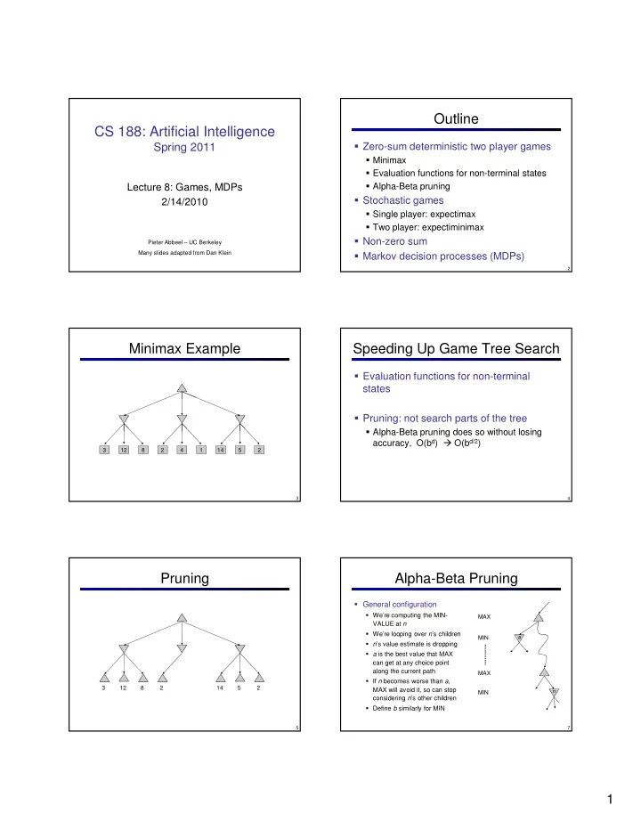
Outline CS 188: Artificial Intelligence Zero-sum deterministic two - PDF document

Outline CS 188: Artificial Intelligence � Zero-sum deterministic two player games Spring 2011 � Minimax � Evaluation functions for non-terminal states � Alpha-Beta pruning Lecture 8: Games, MDPs � Stochastic games 2/14/2010 � Single player: expectimax � Two player: expectiminimax � Non-zero sum Pieter Abbeel – UC Berkeley Many slides adapted from Dan Klein � Markov decision processes (MDPs) 1 2 Minimax Example Speeding Up Game Tree Search � Evaluation functions for non-terminal states � Pruning: not search parts of the tree � Alpha-Beta pruning does so without losing accuracy, O(b d ) � O(b d/2 ) 3 12 8 2 4 1 14 5 2 3 4 Pruning Alpha-Beta Pruning � General configuration � We’re computing the MIN- MAX VALUE at n � We’re looping over n ’s children MIN a � n ’s value estimate is dropping � a is the best value that MAX can get at any choice point along the current path MAX � If n becomes worse than a , 3 12 8 2 14 5 2 MAX will avoid it, so can stop n MIN considering n ’s other children � Define b similarly for MIN 5 7 1

Alpha-Beta Pruning Example Alpha-Beta Pruning Example a=- ∞ Starting a/b b=+ ∞ 3 3 Raising a a=- ∞ a=3 a=3 a=3 b=+ ∞ b=+ ∞ b=+ ∞ b=+ ∞ ≤ 2 ≤ 1 ≤ 2 ≤ 1 3 3 Lowering b a=- ∞ a=- ∞ a=- ∞ a=- ∞ a=3 a=3 a=3 a=3 a=3 a=3 b=+ ∞ b=3 b=3 b=3 b=+ ∞ b=2 b=+ ∞ b=14 b=5 b=1 3 12 2 14 5 1 3 12 2 14 5 1 ≥ 8 ≥ 8 Raising a a is MAX’s best alternative here or above a=- ∞ a=8 a is MAX’s best alternative here or above 8 b=3 8 b=3 b is MIN’s best alternative here or above b is MIN’s best alternative here or above Alpha-Beta Pseudocode Alpha-Beta Pruning Properties � This pruning has no effect on final result at the root � Values of intermediate nodes might be wrong! � Good child ordering improves effectiveness of pruning � Heuristic: order by evaluation function or based on previous search � With “perfect ordering”: � Time complexity drops to O(b m/2 ) � Doubles solvable depth! b � Full search of, e.g. chess, is still hopeless… � This is a simple example of metareasoning (computing v about what to compute) 11 Outline Expectimax Search Trees � What if we don’t know what the � Zero-sum deterministic two player games result of an action will be? E.g., � In solitaire, next card is unknown � Minimax � In minesweeper, mine locations max � In pacman, the ghosts act randomly � Evaluation functions for non-terminal states � Can do expectimax search to � Alpha-Beta pruning chance maximize average score � Chance nodes, like min nodes, � Stochastic games except the outcome is uncertain � Calculate expected utilities � Single player: expectimax � Max nodes as in minimax search � Chance nodes take average 10 10 10 4 9 5 100 7 � Two player: expectiminimax (expectation) of value of children � Non-zero sum � Later, we’ll learn how to formalize the underlying problem as a � Markov decision processes (MDPs) Markov Decision Process 12 13 2

Expectimax Pseudocode Expectimax Quantities def value(s) if s is a max node return maxValue(s) if s is an exp node return expValue(s) if s is a terminal node return evaluation(s) def maxValue(s) values = [value(s’) for s’ in successors(s)] return max(values) 8 4 5 6 def expValue(s) 3 12 9 2 4 6 15 6 0 values = [value(s’) for s’ in successors(s)] weights = [probability(s, s’) for s’ in successors(s)] return expectation(values, weights) 14 15 Expectimax Pruning? Expectimax Search � Chance nodes � Chance nodes are like min nodes, except the outcome is uncertain 1 search ply � Calculate expected utilities � Chance nodes average successor values (weighted) � Each chance node has a probability distribution over its outcomes (called a model) Estimate of true � For now, assume we’re … expectimax value 400 300 3 12 9 2 4 6 15 6 0 given the model (which would require a lot of � Utilities for terminal states … work to compute) � Static evaluation functions … give us limited-depth search 492 362 16 Expectimax for Pacman � Notice that we’ve gotten away from thinking that the ghosts are trying to minimize pacman’s score � Instead, they are now a part of the environment � Pacman has a belief (distribution) over how they will act � Quiz: Can we see minimax as a special case of expectimax? � Quiz: what would pacman’s computation look like if we assumed that the ghosts were doing 1-ply minimax and taking the result 80% of the time, otherwise moving randomly? � If you take this further, you end up calculating belief distributions over your opponents’ belief distributions over your belief distributions, etc… � Can get unmanageable very quickly! 18 19 3

Expectimax Utilities Stochastic Two-Player � E.g. backgammon � For minimax, terminal function scale doesn’t matter � Expectiminimax (!) � We just want better states to have higher evaluations (get the ordering right) � Environment is an � We call this insensitivity to monotonic transformations extra player that moves after each agent � Chance nodes take � For expectimax, we need magnitudes to be meaningful expectations, otherwise like minimax x 2 0 40 20 30 0 1600 400 900 23 Stochastic Two-Player Non-Zero-Sum Utilities � Dice rolls increase b : 21 possible rolls � Similar to with 2 dice minimax: � Backgammon ≈ 20 legal moves � Terminals have utility tuples � Depth 2 = 20 x (21 x 20) 3 = 1.2 x 10 9 � Node values � As depth increases, probability of are also utility tuples reaching a given search node shrinks � Each player � So usefulness of search is diminished maximizes its � So limiting depth is less damaging own utility and propagate (or � But pruning is trickier… back up) nodes � TDGammon uses depth-2 search + from children 1,6,6 7,1,2 6,1,2 7,2,1 5,1,7 1,5,2 7,7,1 5,2,5 � Can give rise very good evaluation function + to cooperation reinforcement learning: and world-champion level play competition dynamically… � 1 st AI world champion in any game! 25 Outline Reinforcement Learning � Basic idea: � Zero-sum deterministic two player games � Receive feedback in the form of rewards � Minimax � Agent’s utility is defined by the reward function � Must learn to act so as to maximize expected rewards � Evaluation functions for non-terminal states � Alpha-Beta pruning � Stochastic games � Single player: expectimax � Two player: expectiminimax � Non-zero sum � Markov decision processes (MDPs) 26 4

Grid World Grid Futures � The agent lives in a grid Deterministic Grid World Stochastic Grid World � Walls block the agent’s path � The agent’s actions do not always X X go as planned: � 80% of the time, the action North E N S W takes the agent North (if there is no wall there) E N S W ? � 10% of the time, North takes the agent West; 10% East � If there is a wall in the direction the agent would have been taken, the agent stays put X X � Small “living” reward each step X X � Big rewards come at the end � Goal: maximize sum of rewards 30 Markov Decision Processes What is Markov about MDPs? � An MDP is defined by: � Andrey Markov (1856-1922) � A set of states s ∈ S � A set of actions a ∈ A � “Markov” generally means that given � A transition function T(s,a,s’) � Prob that a from s leads to s’ the present state, the future and the � i.e., P(s’ | s,a) past are independent � Also called the model � A reward function R(s, a, s’) � For Markov decision processes, � Sometimes just R(s) or R(s’) � A start state (or distribution) “Markov” means: � Maybe a terminal state � MDPs are a family of non- deterministic search problems � Reinforcement learning: MDPs where we don’t know the transition or reward functions 31 Solving MDPs Example Optimal Policies � In deterministic single-agent search problems, want an optimal plan, or sequence of actions, from start to a goal � In an MDP, we want an optimal policy π *: S → A � A policy π gives an action for each state � An optimal policy maximizes expected utility if followed � Defines a reflex agent R(s) = -0.01 R(s) = -0.03 Optimal policy when R(s, a, s’) = -0.03 for all non-terminals s R(s) = -0.4 R(s) = -2.0 35 5