Out line Learning f rom complet e Dat a St at ist ical Learning - PDF document

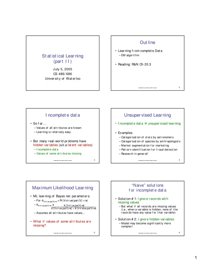
Out line • Learning f rom complet e Dat a St at ist ical Learning – EM algor it hm (part I I ) • Reading: R&N Ch 20.3 J uly 5, 2005 CS 486/ 686 Univer sit y of Wat erloo 2 CS486/686 Lecture Slides (c) 2005 P. Poupart I ncomplet e dat a Unsupervised Learning • So f ar… • I ncomplet e dat a � unsuper vised lear ning – Values of all at t ribut es are known – Learning is relat ively easy • Examples: – Cat egorisat ion of st ars by ast ronomers • But many r eal-wor ld problems have – Cat egorisat ion of species by ant hropologist s hidden var iables (a.k.a lat ent var iables) – Market segment at ion f or market ing – I ncomplet e dat a – Pat t ern ident if icat ion f or f raud det ect ion – Values of some at t ribut es missing – Resear ch in general! 3 4 CS486/686 Lecture Slides (c) 2005 P. Poupart CS486/686 Lecture Slides (c) 2005 P. Poupart “Naive” solut ions Maximum Likelihood Learning f or incomplet e dat a • ML learning of Bayes net paramet er s: • Solut ion # 1: I gnore records wit h – For θ V=t r ue,pa(V)= v = Pr(V=t rue| par (V) = v ) missing values – θ V=t r ue,pa(V)= v = # [V=t rue,pa(V)= v ] – But what if all records are missing values # [V=t rue,pa(V)= v ] + # [V=f alse,pa(V)= v ] (i.e., when a variable is hidden, none of t he records have any value f or t hat variable) – Assumes all at t ribut es have values… • Solut ion # 2: I gnore hidden variables • What if values of some at t r ibut es are – Model may become signif icant ly more missing? complex! 5 6 CS486/686 Lecture Slides (c) 2005 P. Poupart CS486/686 Lecture Slides (c) 2005 P. Poupart 1

Heart disease example “Direct ” maximum likelihood 2 2 2 2 2 2 Smoking Diet Exercise Smoking Diet Exercise • Solut ion 3: maximize likelihood dir ect ly – Let Z be hidden and E observable 54 HeartDisease – h ML = argmax h P( e | h) = argmax h Σ Z P( e , Z | h) 6 6 6 54 162 486 = argmax h Σ Z Π i CPT(V i ) Symptom 1 Symptom 2 Symptom 3 Symptom 1 Symptom 2 Symptom 3 = argmax h log Σ Z Π i CPT(V i ) (b) (a) – Problem: can’t push log past sum t o • a) simpler (i.e., f ewer CPT paramet er s) linear ize pr oduct • b) complex (i.e., lot s of CPT par amet er s) 7 8 CS486/686 Lecture Slides (c) 2005 P. Poupart CS486/686 Lecture Slides (c) 2005 P. Poupart Expect at ion-Maximizat ion (EM) Expect at ion-Maximizat ion (EM) • Solut ion # 4: EM algor it hm • More f ormally: – I nt uit ion: if we new t he missing values, – Appr oximat e maximum likelihood comput ing h ML would be t rival – I t erat ively comput e: h i+1 = argmax h Σ Z P( Z | h i , e ) log P( e , Z | h) • Guess h ML • I t erat e Expect at ion – Expect at ion: based on h ML , comput e expect at ion of t he missing values – Maximizat ion: based on expect ed missing values, comput e new est imat e of h ML Maximizat ion 9 10 CS486/686 Lecture Slides (c) 2005 P. Poupart CS486/686 Lecture Slides (c) 2005 P. Poupart Expect at ion-Maximizat ion (EM) Expect at ion-Maximizat ion (EM) • Derivat ion – log P( e | h) = log [P( e, Z | h) / P( Z | e ,h)] • Log inside sum can linearize product = log P( e, Z | h) – log P( Z | e ,h) – h i+1 = argmax h Σ Z P( Z | h i , e ) log P( e , Z | h) = Σ Z P( Z | e ,h) log P( e,Z | h) = argmax h Σ Z P( Z | h i , e ) log Π j CPT j – Σ Z P( Z | e ,h) log P( Z | e ,h) = argmax h Σ Z P( Z | h i , e ) Σ j log CPT j ≥ Σ Z P( Z | e ,h) log P( e,Z | h) • EM f inds a local maximum of • Monot onic improvement of likelihood Σ Z P(Z| e,h) log P( e, Z | h) – P( e | h i+1 ) ≥ P( e | h i ) which is a lower bound of log P( e | h) 11 12 CS486/686 Lecture Slides (c) 2005 P. Poupart CS486/686 Lecture Slides (c) 2005 P. Poupart 2

Candy Example Candy Example • Suppose you buy t wo bags of candies of • “Bag” var iable is hidden unknown t ype (e.g. f lavour rat ios) • You plan t o eat suf f icient ly many candies of each bag t o lear n t heir t ype • I gnoring your plan, your roommat e mixes bot h bags… • How can you learn t he t ype of each bag despit e being mixed? 13 14 CS486/686 Lecture Slides (c) 2005 P. Poupart CS486/686 Lecture Slides (c) 2005 P. Poupart Unsupervised Clust ering Candy Example • “Class” var iable is hidden • Unknown Par amet er s: – θ i = P(Bag=i) • Naïve Bayes model – θ Fi = P(Flavour=cherry| Bag=i) P ( Bag= 1) – θ Wi = P(Wrapper=red| Bag=i) Bag C – θ Hi = P(Hole=yes| Bag=i) P ( F=cherry | B ) Bag 1 F 1 • When eat ing a candy: 2 F 2 – F, W and H are observable Flavor Wrapper Holes X – B is hidden (a) (b) 15 16 CS486/686 Lecture Slides (c) 2005 P. Poupart CS486/686 Lecture Slides (c) 2005 P. Poupart Candy Example Candy Example • Let t rue par amet er s be: • EM algorit hm – θ =0.5, θ F1 = θ W1 = θ H1 =0.8, θ F2 = θ W2 = θ H2 =0.3 • Guess h 0 : – θ =0.6, θ F1 = θ W1 = θ H1 =0.6, θ F2 = θ W2 = θ H2 =0.4 • Af t er eat ing 1000 candies: • Alt ernat e: W=red W=green – Expect at ion: expect ed # of candies in each H=1 H=0 H=1 H=0 bag F=cherr y 273 93 104 90 – Maximizat ion: new paramet er est imat es F=lime 79 100 94 167 17 18 CS486/686 Lecture Slides (c) 2005 P. Poupart CS486/686 Lecture Slides (c) 2005 P. Poupart 3

Candy Example Candy Example • Expect at ion: expect ed # of candies in • Maximizat ion: relat ive f r equency of each bag each bag – θ 1 = 612/ 1000 = 0.612 – # [Bag=i] = Σ j P(B=i| f j ,w j ,h j ) – Comput e P(B=i| f j ,w j ,h j ) by variable – θ 2 = 388/ 1000 = 0.388 eliminat ion (or any ot her inf erence alg.) • Example: – # [Bag=1] = 612 – # [Bag=2] = 388 19 20 CS486/686 Lecture Slides (c) 2005 P. Poupart CS486/686 Lecture Slides (c) 2005 P. Poupart Candy Example Candy Example • Expect at ion: expect ed # of cherry -1975 -1980 candies in each bag -1985 – # [B=i,F=cherry] = Σ j P(B=i| f j =cherry,w j ,h j ) -1990 Log-likelihood – Comput e P(B=i| f j =cher ry,w j ,h j ) by variable -1995 -2000 eliminat ion (or any ot her inf erence alg.) -2005 -2010 • Maximizat ion: -2015 – θ F 1 = # [B=1,F=cherry] / # [B=1] = 0.668 -2020 – θ F 2 = # [B=2,F=cherry] / # [B=2] = 0.389 -2025 0 20 40 60 80 100 120 Iteration number 21 22 CS486/686 Lecture Slides (c) 2005 P. Poupart CS486/686 Lecture Slides (c) 2005 P. Poupart Next Class Bayesian net works • EM algorit hm f or gener al Bayes net s • Next Class: •Neur al net wor ks • Expect at ion: •Russell and Norvig Sect . 20.5 – # [V i =v ij ,Pa(V i )=pa ik ] = expect ed f requency • Maximizat ion: – θ vij ,paik = # [V i =v ij ,Pa(V i )=pa ik ] / # [Pa(V i )=pa ik ] 23 24 CS486/686 Lecture Slides (c) 2005 P. Poupart CS486/686 Lecture Slides (c) 2005 P. Poupart 4