Operating System Operating System Concepts Concepts - - PDF document

SLIDE 1

1

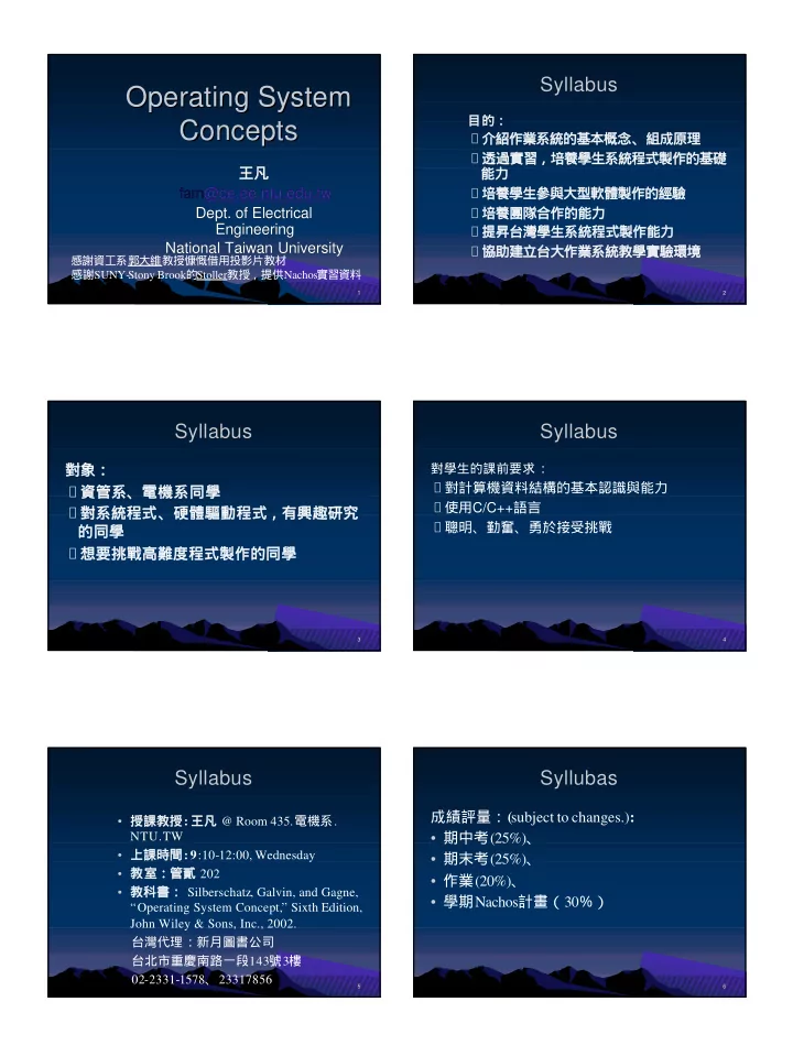
Operating System Operating System Concepts Concepts

王凡 王凡 farn farn@ce.ee.ntu.edu.tw @ce.ee.ntu.edu.tw

• Dept. of Electrical
• Dept. of Electrical

Engineering Engineering National Taiwan University National Taiwan University

感謝資工系郭大維教授慷慨借用投影片教材 感謝SUNY-Stony Brook的Stoller教授，提供Nachos實習資料

2

Syllabus Syllabus

目的：

‧介紹作業系統的基本概念、組成原理 ‧透過實習，培養學生系統程式製作的基礎 能力 ‧培養學生參與大型軟體製作的經驗 ‧培養團隊合作的能力 ‧提昇台灣學生系統程式製作能力 ‧協助建立台大作業系統教學實驗環境

3

Syllabus Syllabus

對象： ‧資管系、電機系同學 ‧對系統程式、硬體驅動程式，有興趣研究 的同學 ‧想要挑戰高難度程式製作的同學

4

Syllabus Syllabus

對學生的課前要求：

‧對計算機資料結構的基本認識與能力 ‧使用C/C++語言 ‧聰明、勤奮、勇於接受挑戰

5

Syllabus Syllabus

• 授課教授: 王凡 @ Room 435.電機系.

NTU.TW

• 上課時間: 9:10-12:00, Wednesday
• 教室：管貳 202
• 教科書： Silberschatz, Galvin, and Gagne,

“Operating System Concept,” Sixth Edition, John Wiley & Sons, Inc., 2002. 台灣代理：新月圖書公司 台北市重慶南路一段143號3樓 02-2331-1578、23317856

6

Syllubas Syllubas

成績評量：(subject to changes.):

• 期中考(25%)、
• 期末考(25%)、
• 作業(20%)、
• 學期Nachos計畫（30％）

SLIDE 2

7

Syllabus Syllabus

‧學期計畫：Nachos作業系統實習 ‧在PC Linux下執行 ‧模擬MIPS硬體架構 ‧目前暫訂兩個部分：

–Thread management –Virtual memory management

8

Syllabus Syllabus

教師與課程網址： http://cc.ee.ntu.edu.tw/~farn 教師e m a i l : f a r n @ c c . e e . n t u . e d u . t w

9

Syllabus Syllabus

預定課程進度 1. 2/19 課程簡介 2. 2/26 第一章 3. 3/5 第二章 4. 3/12 第二章、第三章 5. 3/19 第三章 6. 3/26 第四章、 第一次學期報告介紹：Nachos簡介

10 10

Syllabus Syllabus

預定課程進度 7. 4/2 第四章、 第二次學期計畫報告介紹：

第一階段工作說明，t h r e a d m a n a g e m e n t

8. 4/9 第五章 9. 4/16 期中考

• 10. 4/23

第五章、第六章

• 11. 4/30

第六章

11 11

Syllabus Syllabus

預定課程進度

• 12. 5/7

第六章、第七章 繳交學期報告第一階段工作報告

• 13. 5/14

第七章

• 14. 5/21

第八章 第三次學期報告說明：第二階段工作說 明：virtual memory

• 13. 5/28

第九章

12 12

Syllabus Syllabus

預定課程進度

• 16. 6/4

端午節

• 17. 6/11

第十章

• 18. 6/18

期末考

• 19. 6/25

繳交學期計畫報告

SLIDE 3

13 13

Syllabus Syllabus

‧助教：

–陳佳蘊（資管碩士班一年級） –林仲輝（資管碩士班一年級）

‧助教時間：每週一小時，時間、地點待宣布

14 14

Contents Contents

• 1. Introduction
• 2. Computer-System

Structures

• 3. Operating-System

Structures

• 4. Processes
• 5. Threads
• 6. CPU Scheduling
• 7. Process Synchronization
• 8. Deadlocks
• 9. Memory Management

15 15

Chapter 1. Chapter 1. Introduction Introduction

16 16

Introduction Introduction

• What is an Operating System?

– A basis for application programs – An intermediary between users and hardware

• Amazing variety

– Mainframe, personal computer (PC), handheld computer, embedded computer without user view Convenient vs Efficient

17 17

Computer System Computer System Components Components

• OS – a government/environment

provider Application Programs Operating System Hardware

User User User ................. CPU, I/O devices, memory, etc. compilers, word processors, spreadsheets, Browsers, etc.

18 18

User View User View

• The user view of the computer

varies by the interface being used!

• Examples:

– Personal Computer Ease of use – Mainframe or minicomputer maximization of resource utilization

• Efficiency and fair share

– Workstations compromise between individual usability & resource utilization – Handheld computer individual usability – Embedded computer without user view

SLIDE 4

19 19

System View System View

• A Resource Allocator

– CPU time, Memory Space, File Storage, I/O Devices, Shared Code, Data Structures, and more

• A Control Program

– Control execution of user programs – Prevent errors and misuse

• OS definitions – US Dept.of

Justice against Microsoft in 1998

– The stuff shipped by vendors as an OS – Run at all time

20 20

System Goals System Goals

• Two Conflicting Goals:

– Convenience for the user! – Efficient operation of the computer system! – Safety and security

• We should

– recognize the influences of operating systems and computer architecture on each other – and learn why’s and how ’s of OS by tracing their evolution and predicting what they will become!

21 21

UNIX Architecture UNIX Architecture

terminal controller, terminals, physical memory, device controller, devices such as disks, memory, etc. CPU scheduling, signal handling, virtual memory, paging, swapping, file system, disk drivers, caching/buffering, etc. Shells, compilers, X, application programs, etc. UNIX Kernel interface to the hardware System call interface user user user useruser user user User interface

22 22

Mainframe Systems Mainframe Systems

• The first used to tackle many

commercial and scientific applications!

– 0th Generation – 1940?s – A significant amount of set-up time in the running of a job – Programmer = operator – Programmed in binary assembler (1950) high level language

23 23

Mainframe Mainframe – Batch Systems Batch Systems

• Batches sorted and

submitted by the operator

• Simple batch systems

– Off-line processing ~ Replace slow input device with faster units replace card readers with disks – Resident monitor ~ Automatically transfer control from one job to the next

• loader
• job sequencing
• control card

interpreter User Program Area monitor

24 24

Mainframe Mainframe – Batch Systems Batch Systems

– Spooling (Simultaneous Peripheral Operation On-Line)

~ Replace sequential-access devices with random-access device => Overlap the I/O of one job with the computation of

• thers

e.g. card disk, CPU services, disk printer

– Job Scheduling

card reader disks CPU disks printer

SLIDE 5

25 25

Mainframe Mainframe – Multiprogrammed Multiprogrammed Systems Systems

• Multiprogramming increases

CPU utilization by organizing jobs so that the CPU always has one to execute – Early 1960

– Multiporgrammed batched systems – Job scheduling and CPU scheduling – Goal : efficient use of scarce resources

disk monitor CPU scheduling job1 job2 job3

26 26

Mainframe Mainframe – Time Time-Sharing Sharing Systems Systems

• Time sharing (or

multitasking) is a logical extension of multiprogramming!

– Started in 1960s and become common in 1970s. – An interactive (or hand-

• n) computer system

– Multics, IBM OS/360

disk

• n-line file system

virtual memory sophisticated CPU scheduling job synchronization protection & security ...... and so on

27 27

Desktop Systems Desktop Systems

• Personal Computers (PC’s)

– Appeared in the 1970s. – Goals of operating systems keep changing

• Less-Powerful Hardware & Isolated

Environment Poor Features

– Benefited from the development of mainframe OS’s and the dropping of hardware cost – Advanced protection features

• User Convenience & Responsiveness

28 28

Parallel Systems Parallel Systems

• Tightly coupled: have more than one

processor in close communication sharing computer bus, clock, and sometimes memory and peripheral devices

• Loosely coupled: otherwise
• A Tandem fault-tolerance solution

29 29

Parallel Systems Parallel Systems

• Advantages

– Speedup – Throughput – Lower cost – Economy of Scale – More reliable – Graceful Degradation Fail Soft (detection, diagnosis, correction)

• A Tandem fault-tolerance solution

30 30

Parallel Systems Parallel Systems

• Symmetric multiprocessing model: each

processor runs an identical copy of the OS

• Asymmetric multiprocessing model: a

master- slave relationship

~ Dynamically allocate or pre-allocate tasks ~ Commonly seen in extremely large systems ~ Hardware and software make a difference?

SLIDE 6

31 31

Parallel Systems Parallel Systems

• Trend: the dropping of microporcessor

cost OS functions are offloaded to slave processors (back-ends)

32 32

Distributed Systems Distributed Systems

• Definition: Loosely-Coupled Systems –

processors do not share memory or a clock

– Heterogeneous vs Homogeneous

• Advantages or Reasons

– Resource sharing: computation power, peripheral devices, specialized hardware – Computation speedup: distribute the computation among various sites – load sharing – Reliability: redundancy reliability

33 33

Distributed Systems Distributed Systems

• Distributed systems depend on

networking for their functionality.

– Networks vary by the protocols used.

• TCP/IP, ATM, etc.

– Types – distance

• Local-area network (LAN)
• Wide-area network (WAN)
• Metropolitan-area network (MAN)
• Small-area network – distance of few feet

– Media – copper wires, fiber strands, satellite wireless transmission, infrared communication,etc.

34 34

Distributed Systems Distributed Systems

• Client-Server Systems

– Compute-server systems – File-server systems

• Peer-to-Peer Systems

– Network connectivity is an essential component.

• Network Operating Systems

– Autonomous computers – A distributed operating system – a single OS controlling the network.

35 35

Clustered Systems Clustered Systems

• Definition: Clustered computers which

share storage and are closely linked via LAN networking.

• Advantages: high availability,

performance improvement, etc.

• Types

– Asymmetric/symmetric clustering – Parallel clustering – multiple hosts that access the same data on the shared storage. – Global clusters

• Distributed Lock Manager (DLM)

36 36

Real Real-Time Systems Time Systems

• Definition: A real-time system is a

computer system where a timely

response by the computer to external stimuli is vital!

• Hard real-time system: The

system has failed if a timing constraint, e.g. deadline, is not met.

– All delays in the system must be bounded. – Many advanced features are

SLIDE 7

37 37

Real Real-Time Systems Time Systems

• Soft real-time system: Missing a timing

constraint is serious, but does not necessarily result in a failure unless it is excessive

– A critical task has a higher priority. – Supported in most commercial OS.

• Real-time means on-time instead of fast

38 38

Real Real-Time Systems Time Systems

• Applications

– Air traffic control – Space shuttle – Navigation – Multimedia systems – Industrial control systems – Home appliance controller – Nuclear power plant

Virtual reality Games User interface Vision and speech recognition (approx. 100 ~ 200ms) PDA, telephone system And more

39 39

Handheld Systems Handheld Systems

• Handheld Systems

– E.g., Personal Digital Assistant (PDA)

• New Challenges – convenience vs

portability

– Limited Size and Weight – Small Memory Size

• No Virtual Memory

– Slow Processor

• Battery Power

– Small display screen

• Web-clipping

40 40

Feature Migration Feature Migration

• MULTIplexed Information and

Computing Services (MULTICS)

– 1965-1970 at MIT as a utility

• UNIX

– Since 1970 on PDP

• 11
• Recent OS’s

– MS Windows, IBM OS/2, MacOS X

• OS features being scaled down to

fit PC’s

– Personal Workstations – large PC’s

41 41

Computing Environments Computing Environments

• Traditional Computing

– E.g., typical office environment

• Web-Based Computing

– Web Technology

• Portals, network computers, etc.

– Network connectivity – New categories of devices

• Load balancers

42 42

Computing Environments Computing Environments

• Embedded Computing

– Car engines, robots, VCR’s, home automation – Embedded OS’s often have limited features.

SLIDE 8

43 43

Contents Contents

• 1. Introduction
• 2. Computer-System

Structures

• 3. Operating-System

Structures

• 4. Processes
• 5. Threads
• 6. CPU Scheduling
• 7. Process Synchronization
• 8. Deadlocks
• 9. Memory Management

44 44

Chapter 2 Chapter 2 Computer Computer-System System Structure Structure

45 45

Computer Computer-System Structure System Structure

• Objective: General knowledge of

the structure of a computer system.

printer CPU printer controller memory controller disk controller memory tape-drive controller disks tape drivers

Device controllers: synchronize and manage access to devices.

46 46

Booting Booting

• Bootstrap program:

– Initialize all aspects of the system, e.g., CPU registers, device controllers, memory, etc. – Load and run the OS

• Operating system: run init to

initialize system processes, e.g., various daemons, login processes, after the kernel has been bootstrapped. (/etc/rc* & init

• r /sbin/rc* & init)

47 47

Interrupt Interrupt

• Hardware interrupt, e.g. services

requests of I/O devices

• Software interrupt, e.g. signals,

invalid memory access, division by zero, system calls, etc – (trap)

• Procedures: generic handler or

interrupt vector (MS-DOS,UNIX)

process execution interrupt handler return

48 48

Interrupt Handling Procedure Interrupt Handling Procedure

• Saving of the address of the

interrupted instruction: fixed locations

• r stacks
• Interrupt disabling or enabling issues:

lost interrupt?! prioritized interrupts masking

interrupted process system stack fixed address per interrupt type interrupted address, registers ...... handler

SLIDE 9

49 49

Interrupt Handling Interrupt Handling Procedure Procedure

• Interrupt Handling

Save interrupt information OS determine the interrupt type (by polling) Call the corresponding handlers Return to the interrupted job by the restoring important information (e.g., saved return addr. program counter)

indexed by a unique device number Interrupt Vector 1 n

• Interrupt Handlers

(Interrupt Service Routines)

50 50

I/O Structure I/O Structure

• The device drivers are responsible of

moving data between the peripheral devices and their local buffer storages.

printer CPU printer controller memory controller DMA memory tape-drive controller disk tape drivers

registers buffers registers buffers

51 51

I/O Structure I/O Structure

• I/O operation
• a. CPU sets up specific controller registers

within the controller.

• b. Read: devices controller buffers

memory Write: memory controller buffers devices

• c. Notify the completion of the operation by

triggering an interrupt

52 52

I/O Types I/O Types

I/O system call wait till the completion

• wait

wait instruction (idle till interrupted)

• looping
• polling
• wait for an interrupt
• r
• r
• a. Synchronous I/O

– Issues: overlapping of computations and IO activities, concurrent I/O activities, etc. Loop: jmp Loop

53 53

I/O types I/O types

• b. Asynchronous I/O

sync wait till the completion wait mechanisms!! *efficiency

54 54

I/O Types I/O Types

Hardware data transfer Interrupt handler Device driver Requesting process Hardware data transfer Interrupt handler Device driver Requesting process user Kernel user Kernel Synchronous I/O Time Time Asynchronous I/O wait

SLIDE 10

55 55

I/O Types I/O Types

• A Device-Status Table Approach

card reader 1 status: idle line printer 3 status: busy disk unit 3 status: idle ........ Request

• addr. 38596

len?1372 Request file:xx Record

• Addr. len

Request file:yy Record

• Addr. len

process 1 process 2

• Tracking of many

I/O requests

• type-ahead service

56 56

DMA DMA

• Goal: Release CPU from handling

excessive interrupts!

– E.g. 9600-baud terminal

2-microsecond service / 1000 microseconds

High-speed device:

2-microsecond service / 4 microseconds

• Procedure

– Execute the device driver to set up the registers of the DMA controller. – DMA moves blocks of data between the memory and its own buffers. – Transfer from its buffers to its devices. – Interrupt the CPU when the job is done.

57 57

Storage Structure Storage Structure

• Access time: a

cycle

• Access time:

several cycles

• Access time:

many cycles

memory Magnetic Disks registers cache CD-ROMs/DVDs Jukeboxes Tertiary Storage

• removable media

Secondary Storage

• nonvolatile storage

HW-Managed SW-Managed

Primary Storage

• volatile storage

CPU * Differences: Size, Cost, Speed, Volatility

58 58

Memory Memory

• Processor can have direct

access!

• Intermediate storage for data in

the registers of device controllers

• Memory-Mapped I/O (PC &

Mac)

(1)Frequently used devices (2)Devices must be fast, such as video controller, or special I/O instructions is used to move data between memory & device

R 1 R 2 R 3 . . .

Memory Device Controller

59 59

Magnetic disks Magnetic disks

• Transfer

Rate

• Random-

Access Time

– Seek time in x ms – Rotational latency in y ms

• 60~200

times/sec spindle sector cylinder platter r/w head disk arm arm assembly track

60 60

Magnetic Disks Magnetic Disks

• Disks

– Fixed-head disks:

• More r/w heads v.s. fast track switching

– Moving-head disks (hard disk) – Primary concerns:

• Cost, Size, Speed

– Computer host controller disk controller disk drives (cache disks)

• Floppy disk

– slow rotation, low capacity, low density, but less expensive

• Tapes: backup or data transfer bet

SLIDE 11

61 61

Storage Hierarchy Storage Hierarchy

register Main Memory Electronic Disk Magnetic Disk Optical Disk Cache Magnetic Tape Cost

High hitting rate

• instruction & data cache
• combined cache

Faster than magnetic disk – nonvolatile?! Alias: RAM Disks Sequential Access XX GB/350F

Speed Volatile Storage

62 62

Storage Hierarchy Storage Hierarchy

• Caching

– Information is copied to a faster storage system on a temporary basis – Assumption: Data will be used again soon.

• Programmable registers, instr. Cache, etc.
• Cache Management

– Cache Size and the Replacement Policy

• Movement of Information Between

Hierarchy

– Hardware Design & Controlling

63 63

Storage Hierarchy Storage Hierarchy

• Coherency and Consistency

– Among several storage levels (vertical)

• Multitasking vsunitasking

– Among units of the same storage level , (horizontal), e.g. cache coherency

• Multiprocessor or distributed systems

Memory Cache CPU Memory cache

CPU

64 64

Hardware Protection Hardware Protection

• Goal:

– Prevent errors and misuse!

• E.g., input errors of a program in a

simple batch operating system

• E.g., the modifications of data and code

segments of another process or OS

• Dual-Mode Operations – a mode

bit

– User-mode executions except those after a trap or an interrupt occurs. – Monitor-mode (system mode, privileged mode, supervisor mode)

• Privileged instruction:machine

65 65

Hardware Protection Hardware Protection

• System Calls – trap to OS for

executing privileged instructions.

• Resources to protect

– I/O devices, Memory, CPU

• I/O Protection (I/O devices are

scare resources!)

– I/O instructions are privileged.

• User programs must issue I/O through

OS

• User programs can never gain control
• ver the computer in the system mode.

66 66

Hardware Protection Hardware Protection

• Memory Protection

– Goal: Prevent a user program from modifying the code or data structures of either the OS or other users! – Instructions to modify the memory space for a process are privileged.

kernel job1 …… job2 …… Limit register Base register Check for every memory address by hardware

SLIDE 12

67 67

Hardware Protection Hardware Protection

• CPU Protection

– Goal

• Prevent user programs from sucking

up CPU power!

– Use a timer to implement time- sharing or to compute the current time.

• Instructions that modify timers are

privileged.

– Computer control is turned over to OS for every time-slice of time!

• Terms: time-sharing, context switch

68 68

Network Structure Network Structure

• Local-Area Network (LAN)

– Characteristics:

• Geographically distributed in a small

area, e.g., an office with different computers and peripheral devices.

• More reliable and better speed

– High-quality cables, e.g., twisted pair cables for 10BaseT Ethernet or fiber optic cables for 100BaseT Ethernet

– Started in 1970s – Configurations: multiaccess bus, ring, star networks (with gateways)

69 69

Network Structure Network Structure

• Wide-Area Network (WAN)

– Emerged in late 1960s (Arpanet in 1968)

• World Wide Web (WWW)

– Utilize TCP/IP over ARPANET/Internet.

• Definition of “Intranet”: roughly speaking for any network under
• ne authorization, e.g., a company or a school.
• Often in a Local Area Network (LAN), or connected LAN’s.
• Having one (or several) gateway with the outside world.
• In general, it has a higher bandwidth because of a LAN.

70 70

Network Structure Network Structure – WAN WAN

gateway gateway TARNET TARNET HINET HINET Intranet A Intranet A Intranet A Intranet A Intranet Intranet Intranet Intranet router Intranet Intranet

71 71

Network Structure Network Structure – WAN WAN

• Router

– With a Routing table

• Use some routing protocol, e.g., to maintain

network topology by broadcasting.

– Connecting several subnets (of the same IP-

• r-higher-layer protocols) for forwarding

packets to proper subnets.

• Gateway

– Functionality containing that of routers. – Connecting several subnets (of different or the same networks, e.g., Bitnet and Internet)for forwarding packets to proper

72 72

Network Structure Network Structure – WAN WAN

• Connections between

networks

– T1: 1.544 mbps, T3: 45mbps (28T1)

• Telephone-system services over

T1

• Modems

– Conversion of the analog signal and digital signal

SLIDE 13

73 73

Network Layers in Linux Network Layers in Linux

PPP SLIP Ethernet Internet Protocol (IP)

Network Layer

ARP TCP UDP INET sockets BSD sockets Kernel Applications applications

74 74

TCP/IP TCP/IP

• IP Address:

– 140.123.101.1

• 256*256*256*256 combinations

– 140.123 -> Network Address – 101.1 -> Host Address

• Subnet:

– 140.123.101 and 140.123.102

– Mapping of IP addresses and host names

• Static assignments: /etc/hosts
• Dynamic acquisition: DNS (Domain Name Server)

– /etc/resolv.confg

• If /etc/hosts is out- of-date, re-check it up with DNS!

– Domain name: cs.ccu.edu.tw as a domain name for 140.123.100, 140.123. 101, and 140.123.103

75 75

TCP/IP TCP/IP

• Transmission Control Protocol (TCP)

– Reliable point-to-point packet transmissions. – Applications which communicate over TCP/IP with each another must provide IP addresses and port numbers.

• /etc/services
• Port# 80 for a web server.
• User Datagram Protocol (UDP)

– Unreliable point-to-point services.

• Both are over IP.

76 76

TCP/IP TCP/IP

• Mapping of Ethernet physical

addresses and IP addresses

– Each Ethernet card has a built-in Ethernet physical address, e.g., 08-01-2b-00-50-A6. – Ethernet cards only recognize frames with their physical addresses. – Linux uses ARP (Address Resolution Protocol) to know and maintain the mapping.

• Broadcast requests over Ethernet for IP

address resolution over ARP.

• Machines with the indicated IP addresses

reply with their Ethernet physical addresses.

77 77

TCP/IP TCP/IP

TCP header + Data IP header Data Ethernet header Data An Ethernet frame An IP packet A TCP packet

• Each IP packet has an indicator of which protocol used, e.g., TCP or UDP

78 78

Contents Contents

• 1. Introduction
• 2. Computer-System

Structures

• 3. Operating-System

Structures

• 4. Processes
• 5. Threads
• 6. CPU Scheduling
• 7. Process Synchronization
• 8. Deadlocks
• 9. Memory Management

SLIDE 14

79 79

Chapter 3 Chapter 3 Operating Operating-System System Structures Structures

80 80

Operating Operating-System System Structures Structures

• Goals: Provide a way to

understand an operating systems

– Services – Interface – System Components

• The type of system desired is the

basis for choices among various algorithms and strategies!

81 81

System Components System Components – Process Process Management Management

• Process Management

– Process: An Active Entity

• Physical and Logical Resources

– Memory, I/O buffers, data, etc.

• Data Structures Representing Current

Activities:

Program Counter Stack Data Section CPU Registers …. And More

Program (code) +

82 82

System Components System Components – Process Process Management Management

• Services

– Process creation and deletion – Process suspension and resumption – Process synchronization – Process communication – Deadlock handling

83 83

System Components System Components – Main Main- Memory Management Memory Management

• Memory: a large array of words or bytes, where

each has its own address

• OS must keep several programs in memory to

improve CPU utilization and user response time

• Management algorithms depend on the

hardware support

• Services

– Memory usage and availability – Decision of memory assignment – Memory allocation and deallocation

84 84

System Components System Components – File File Management Management

• Goal:

– A uniform logical view of information storage – Each Medium controlled by a device

• Magnetic tapes, magnetic disks, optical

disks, etc.

• OS provides a logical storage unit:

File

– Formats:

• Free form or being formatted rigidly.

– General Views:

• A sequence of bits, bytes, lines, records

SLIDE 15

85 85

System Components System Components – File File Management Management

• Services

– File creation and deletion – Directory creation and deletion – Primitives for file and directory manipulation – Mapping of files onto secondary storage – File Backup

* Privileges for file access control

86 86

System Components System Components – I/O I/O System Management System Management

• Goal:

– Hide the peculiarities of specific hardware devices from users

• Components of an I/O System

– A buffering, caching, and spooling system – A general device-driver interface – Drivers

87 87

System Components System Components – Secondary Secondary-Storage Storage Management Management

• Goal:

– On-line storage medium for programs & data

• Backup of main memory
• Services for Disk Management

– Free-space management – Storage allocation, e.g., continuous allocation – Disk scheduling, e.g., FCFS

88 88

System Components System Components – Networking Networking

• Issues

– Resources sharing – Routing & connection strategies – Contention and security

• Network access is usually

generalized as a form of file access

– World-Wide-Web over file-transfer protocol (ftp), network file-system (NFS), and hypertext transfer protocol (http)

89 89

System Components System Components – Protection System Protection System

• Goal

– Resources are only allowed to accessed by authorized processes.

• Protected Resources

– Files, CPU, memory space, etc.

• Services

– Detection & controlling mechanisms – Specification mechanisms

90 90

System Components System Components – Command Command-Interpreter Interpreter system system

• Command Interpreter

– Interface between the user and the

• perating system

– Friendly interfaces

• Command-line-based interfaces or

mused-based window-and-menu interface

– e.g., UNIX shell and command.com in MS-DOS

Get the next command Execute the command User-friendly?

SLIDE 16

91 91

Operation Operation-System Services System Services

• Program Execution

– Loading, running, terminating, etc

• I/O Operations

– General/special operations for devices:

• Efficiency & protection
• File-System Manipulation

– Read, write, create, delete, etc

• Communications

– Intra-processor or inter-processor communication – shared memory or

92 92

Operation Operation-System Services System Services

• Error Detection

– Possible errors from CPU, memory, devices, user programs Ensure correct & consistent computing

• Resource Allocation

– Utilization & efficiency

• Accounting
• Protection & Security
• user convenience or system efficiency!

93 93

Operation Operation-System Services System Services

• System calls

– Interface between processes & OS

• How to make system calls?

– Assemble-language instructions or subroutine/functions calls in high- level language such as C or Perl?

• Generation of in-line instructions or a

call to a special run-time routine.

• Example: read and copy of a file!

– Library Calls vs System Calls

94 94

Operation Operation-System Services System Services

• How a system call
• ccurs?

– Types and information

• Parameter Passing

– Registers – Registers pointing to blocks

• Linux

– Stacks

x: parameters for call load address x system call 13

x

register use parameters from table x

Code for System Call 13

95 95

Operation Operation-System Services System Services

• System Calls

– Process Control – File Management – Device Management – Information Maintenance – Communications

96 96

Operation Operation-System Services System Services

• Process & Job Control

– End (normal exit) or abort (abnormal)

• Error level or no

– Load and execute

• How to return control?

– e.g., shell load & execute commands

– Creation and/or termination of processes

• Multiprogramming?

SLIDE 17

97 97

Operation Operation-System Services System Services

• Process & Job Control

(continued)

– Process Control

• Get or set attributes of processes

– Wait for a specified amount of time or an event

• Signal event

– Memory dumping, profiling, tracing, memory allocation & de-allocation

98 98

Operation Operation-System Services System Services

• Examples: MS-DOS & UNIX

kernel command interpreter process free memory kernel interpreter process B free memory process A

99 99

Operation Operation-System Services System Services

• File Management

– Create and delete – Open and close – Read, write, and reposition (e.g., rewinding)

• lseek

– Get or set attributes of files – Operations for directories

100 100

Operation Operation-System Services System Services

• Device management

– Request or release

• Open and close of special files
• Files are abstract or virtual devices.

– Read, write, and reposition (e.g., rewinding) – Get or set file attributes – Logically attach or detach devices

101 101

Operation Operation-System Services System Services

• Information maintenance

– Get or set date or time – Get or set system data, such as the amount of free memory

• Communication

– Message Passing

• Open, close, accept connections

– Host ID or process ID

• Send and receive messages
• Transfer status information

– Shared Memory

• Memory mapping & process synchronization

102 102

Operation Operation-System Services System Services

• Shared Memory

– Max Speed & Comm Convenience

• Message Passing

– No Access Conflict & Easy Implementation

kernel Process A Process B kernel Process A Process B

Shared Memory

M M M

SLIDE 18

103 103

System Programs System Programs

• Goal:

– Provide a convenient environment for program development and execution

• Types

– File Management, e.g., rm. – Status information, e.g., date. – File Modifications, e.g., editors. – Program Loading and Executions, e.g., loader. – Communications, e.g., telnet.

104 104

System Programs System Programs – Command Command Interpreter Interpreter

• Two approaches:

– Contain codes to execute commands

• Fast but the interpreter tends to be

big!

• Painful in revision!

del cd

105 105

System Programs System Programs – Command Command Interpreter Interpreter

• Implement commands as

system programs Search exec files which corresponds to commands (UNIX) – Issues

• a. Parameter Passing

– Potential Hazard: virtual memory

• b. Being Slow
• c. Inconsistent Interpretation of

Parameters

106 106

System Structure System Structure – MS MS-DOS DOS

• MS-DOS Layer Structure

Application program Resident system program MS-DOS device drivers ROM BIOS device drivers

107 107

System Structure System Structure – UNIX UNIX

terminal controller, terminals, physical memory, device controller, devices such as disks, memory, etc. CPU scheduling, signal handling, virtual memory, paging, swapping, file system, disk drivers, caching/buffering, etc. Shells, compilers, X, application programs, etc. UNIX Kernel interface to the hardware System call interface user user user useruser user user User interface

108 108

System Structure System Structure

• A Layered Approach – A Myth

Advantage: Modularity ~ Debugging & Verification Difficulty: Appropriate layer definitions, less efficiency due to overheads！

Layer M Layer M-1

hidden

• ps

new

• ps

existing

• ps

SLIDE 19

109 109

System Structure System Structure

• A Layer Definition Example:

L5 User programs L4 I/O buffering L3 Operator-console device driver L2 Memory management L1 CPU scheduling L0 Hardware

110 110

System Structure System Structure – OS/2 OS/2

• OS/2 Layer Structure

Application Application Application Subsystem Subsystem Subsystem Device driver Device driver Device driver Application-program Interface

‧memory management

System kernel

‧task scheduling ‧device management * Some layers of NT were from user space to kernel space in NT4.0

111 111

System Structure System Structure – Microkernels Microkernels

• The concept of microkernels was

proposed in CMU in mid 1980s (Mach).

– Moving all nonessential components from the kernel to the user or system programs! – No consensus on services in kernel

• Mostly on process and memory

management and communication

• Benefits:

– Ease of OS service extensions portability, reliability, secutrity

112 112

System Structure System Structure – Microkernels Microkernels

• Examples

– Microkernels: True64UNIX (Mach kernel), MacOS X (Mach kernel), QNX (msg passing, proc scheduling, HW interrupts, low - level networking) – Hybrid structures: Windows NT

kernel

OS/2 Applications OS/2 Server POSIX Applications POSIX Server Win32 Applications Win32 Server

113 113

Virtual Machine Virtual Machine

• Virtual Machines: provide an interface

that is identical to the underlying bare hardware

interface processes processes processes processes kernel kernel kernel hardware virtual machine implementation hardware kernel VM1 VM2 VM3

114 114

Virtual Machine Virtual Machine

• Implementation Issues:

– Emulation of Physical Devices

• E.g., Disk Systems

– An IBM minidisk approach

– User/Monitor Modes

• (Physical) Monitor Mode

– Virtual machine software

• (Physical) User Mode

– Virtual monitor mode & Virtual user mode

SLIDE 20

115 115

Virtual Machine Virtual Machine

virtual user mode virtual monitor mode monitor mode

processes processes processes

kernel 1 kernel 2 kernel 3 virtual machine software hardware

P1/VM1 system call Trap Service for the system call Set program counter & register contents, & then restart VM1 Simulate the effect of the I/O instruction Restart VM1 Finish service

time

116 116

Virtual Machine Virtual Machine

• Disadvantages:

– Slow!

• Execute most instructions directly on the

hardware

–No direct sharing of resources

• Physical devices and

communications

* I/O could be slow (interpreted) or fast (spooling)

117 117

Virtual Machine Virtual Machine

• Advantages:

– Complete Protection – Complete Isolation！ – OS Research & Development

• System Development Time

– Extensions to Multiple Personalities, such as Mach (software emulation)

• Emulations of Machines and OS’s, e.g.,

Windows over Linux

118 118

Virtual Machine Virtual Machine – Java Java

• Sun Microsystems in late 1995

– Java Language and API Library – Java Virtual Machine (JVM)

• Class loader (for

bytecode .class files)

• Class verifier
• Java interpreter

–An interpreter, a just-in-time (JIT) compiler, hardware

class loader verifier java interpreter

host system

java .class files

119 119

Virtual Machine Virtual Machine – Java Java

• JVM

– Garbage collection

• Reclaim unused objects

– Implementation being specific for different systems

• Programs are architecture neutral

and portable

class loader verifier java interpreter

host system

java .class files

120 120

System Design & System Design & Implementation Implementation

• Design Goals & Specifications:

– User Goals, e.g., ease of use – System Goals, e.g., reliable

• Rule 1: Separation of Policy &

Mechanism

– Policy：What will be done? – Mechanism ：How to do things? – Example: timer construct and time slice

• Two extreme cases:

SLIDE 21

121 121

System Design & System Design & Implementation Implementation

• OS Implementation in High-

Level Languages

– E.g., UNIX, OS/2, MS NT, etc. – Advantages:

• Being easy to understand & debug
• Being written fast, more compact,

and portable

– Disadvantages:

• Less efficient but more storage for

code

122 122

System Generation System Generation

• SYSGEN (System Generation)

– Ask and probe for information concerning the specific configuration of a hardware system

• CPU, memory, device, OS options, etc.

No recompilation Recompilation & completely Linking of

• f a modified

table-driven modules for source code selected OS

• Issues

– Size, Generality, Ease of modification

123 123

Contents Contents

• 1. Introduction
• 2. Computer-System

Structures

• 3. Operating-System

Structures

• 4. Processes
• 5. Threads
• 6. CPU Scheduling
• 7. Process Synchronization
• 8. Deadlocks
• 9. Memory Management

124 124

Chapter 4 Chapter 4 Processes Processes

125 125

Processes Processes

• Objective:

– Process Concept & Definitions

• Process Classification:

– Operating system processes executing system code – User processes executing system code – User processes executing user code

126 126

Processes Processes

• Example: Special Processes in Unix

– PID 0 – Swapper (i.e., the scheduler)

• Kernel process
• No program on disks correspond to this

process

– PID 1 – init responsible for bringing up a Unix system after the kernel has been

• bootstrapped. (/etc/rc* & init or /sbin/rc* &

init)

• User process with superuser privileges

– PID 2 - pagedaemon responsible for paging

SLIDE 22

127 127

Processes Processes

• Process

– A Basic Unit of Work from the Viewpoint

• f OS

– Types:

• Sequential processes: an activity resulted from

the execution of a program by a processor

• Multi-thread processes

– An Active Entity

• Program Code – A Passive Entity
• Stack and Data Segments

– The Current Activity

• PC, Registers , Contents in the Stack and Data

Segments

128 128

Processes Processes

• Process State

new ready waiting

terminated

running

admitted interrupt scheduled exit I/O or event wait I/O or event completion

129 129

Processes Processes

• Process Control Block (PCB)

– Process State – Program Counter – CPU Registers – CPU Scheduling Information – Memory Management Information – Accounting Information – I/O Status Information

130 130

Processes Processes

• PCB: The repository for any

information that may vary from process to process

pointer process state pc register 1 2 PCB[] NPROC -1

131 131

Processes Processes

• Process Control Block (PCB) – An Unix

Example

– proc[i]

• Everything the system must know when the

process is swapped out.

– pid, priority, state, timer counters, etc.

– .u

• Things the system should know when process

is running

– signal disposition, statistics accounting, files[], etc.

132 132

Processes Processes

• Example: 4.3BSD

text structure proc[i] entry page table Code Segment Data Segment PC heap user stack argv, argc,… sp .u

per-process kernel stack p_textp x_caddr p_p0br u_proc p_addr Red Zone

SLIDE 23

133 133

Processes Processes

• Example: 4.4BSD

proc[i] entry

process grp

…

file descrptors

VM space region lists page table Code Segment Data Segment heap user stack argv, argc,… .u

per-process kernel stack p_p0br u_proc p_addr

134 134

Process Scheduling Process Scheduling

• The goal of multiprogramming

– Maximize CPU/resource utilization!

• The goal of time sharing

– Allow each user to interact with his/her program!

PCB1 PCB2

head tail head tail head tail

PCB3 ready queue disk unit 0 tape unit 1

135 135

Process Scheduling Process Scheduling – A A Queueing Queueing Diagram Diagram

ready queue dispatch CPU I/O I/O queue I/O request

time slice expired

fork a child

wait for an interrupt interrupt occurs child executes child terminate

136 136

Process Scheduling Process Scheduling – Schedulers Schedulers

• Long-Term (/Job) Scheduler

– Goal: Select a good mix of I/O-bound and CPU-bound process

– Remarks：

• 1. Control the degree of multiprogramming
• 2. Can take more time in selecting processes

because of a longer interval between executions

• 3. May not exist physically

CPU Memory

Job pool

137 137

Process Scheduling Process Scheduling – Schedulers Schedulers

• Short-Term (/CPU) Scheduler

– Goal：Efficiently allocate the CPU to one of the ready processes according to some criteria.

• Mid-Term Scheduler

– Swap processes in and out memory to control the degree of multiprogramming

138 138

Process Scheduling Process Scheduling – Context Context Switches Switches

• Context Switch ~ Pure

Overheads

– Save the state of the old process and load the state of the newly scheduled process.

• The context of a process is usually reflected in

PCB and others, e.g., .u in Unix.

• Issues：

– The cost depends on hardware support

• e.g. processes with multiple register sets or

computers with advanced memory management.

– Threads, i.e., light-weight process (LWP),

SLIDE 24

139 139

Operations on Processes Operations on Processes

• Process Creation &

Termination

– Restrictions on resource usage – Passing of Information – Concurrent execution

root pagedaemon swapper init user1 user2 user3

140 140

Operations on Processes Operations on Processes

• Process Duplication

– A copy of parent address space + context is made for child, except

the returned value from fork()：

• Child returns with a value 0
• Parent returns with process id of child

– No shared data structures between parent and child communicate via shared files, pipes, etc. – Use execve() to load a new program – fork() vs vfork() (Unix)

141 141

Operations on Processes Operations on Processes

• Example:

… if ( pid = fork() ) == 0) { /* child process */ execlp(“/bin/ls”, “ls”, NULL); } else if (pid < 0) { fprintf(stderr, “Fork Failed”); exit(-1); } else { /* parent process */ wait(NULL); }

142 142

Operations on Processes Operations on Processes

• Termination of Child Processes

– Reasons:

• Resource usages, needs, etc.

– Kill, exit, wait, abort, signal, etc.

• Cascading Termination

143 143

Cooperating Processes Cooperating Processes

• Cooperating processes can affect
• r be affected by the other

processes

– Independent Processes

• Reasons:

– Information Sharing, e.g., files – Computation Speedup, e.g., parallelism. – Modularity, e.g., functionality dividing

144 144

Cooperating Processes Cooperating Processes

• A Consumer-Producer Example:

– Bounded buffer or unbounded buffer

• Supported by inter-process

communication (IPC) or by hand coding z 1 2 n-1 n-2 in

• ut

buffer[0…n-1] Initially, in=out=0；

SLIDE 25

145 145

Cooperating Processes Cooperating Processes

Producer:

while (1) { /* produce an item nextp */ while (((in+1) % BUFFER_SIZE) ==

• ut)

; /* do nothing */ buffer[ in ] = nextp; in = (in+1) % BUFFER_SIZE; }

146 146

Cooperating Processes Cooperating Processes

Consumer:

while (1) {

while (in == out) ; /* do nothing */ nextc = buffer[ out ];

• ut = (out+1) % BUFFER_SIZE ;

/* consume the item in nextc */ }

147 147

Interprocess Interprocess Communication Communication

• Why Inter-Process Communication (IPC)?

– Exchanging of Data and Control Information!

• Why Process Synchronization?

– Protect critical sections! – Ensure the order of executions!

148 148

Interprocess Interprocess Communication Communication

• IPC

– Shared Memory – Message Passing

• Logical Implementation of

Message Passing

– Fixed/variable msg size, symmetric/asymmetric communication, direct/indirect communication, automatic/explicit buffering, send by copy or reference, etc.

149 149

Interprocess Interprocess Communication Communication

• Classification of Communication by

Naming

– Processes must have a way to refer to each

• ther!

– Types

• Direct Communication
• Indirect Communication

150 150

Interprocess Interprocess Communication Communication – Direct Communication Direct Communication

• Process must explicitly name the

recipient or sender of a communication

– Send(P, msg), Receive(Q, msg)

• Properties of a Link:
• a. Communication links are established

automatically.

• b. Two processes per a link
• c. One link per pair of processes
• d. Bidirectional or unidirectional

SLIDE 26

151 151

Interprocess Interprocess Communication Communication – Direct Communication Direct Communication

• Issue in Addressing:

– Symmetric or asymmetric addressing

Send(P, msg), Receive(id, msg)

• Difficulty:

– Process naming vs modularity

152 152

Interprocess Interprocess Communication Communication – Indirect Indirect Communication Communication

• Two processes can communicate
• nly if the process share a

mailbox (or ports)

• Properties:
• 1. A link is established between a pair of

processes only if they share a mailbox.

• 2. n processes per link for n >= 1.
• 3. n links can exist for a pair of processes

for n >=1. A A send(A, msg)=> =>receive(A, msg)

153 153

Interprocess Interprocess Communication Communication –Indirect Indirect Communication Communication

• Issues:
• a. Who is the recipient of a message?
• b. Owners vs Users
• Process owner as the sole recipient?
• OS Let the creator be the owner?

Privileges can be passed? Garbage collection is needed? P1 msgs ? P2 P3

154 154

Interprocess Interprocess Communication Communication – Synchronization Synchronization

• Blocking or Nonblocking

(Synchronous versus Asynchronous)

– Blocking send – Nonblocking send – Blocking receive – Nonblocking receive

• Rendezvous – blocking send &

receive

155 155

Interprocess Interprocess Communication Communication – Buffering Buffering

• The Capacity of a Link = the # of

messages could be held in the link.

– Zero capacity(no buffering)

• Msg transfer must be synchronized – rendezvous!

– Bounded capacity

• Sender can continue execution without waiting till the

link is full

– Unbounded capacity

• Sender is never delayed!
• The last two items are for asynchronous

communication and may need acknowledgement

156 156

Interprocess Interprocess Communication Communication – Buffering Buffering

• Special cases:
• a. Msgs may be lost if the receiver can not

catch up with msg sending synchronization

• b. Senders are blocked until the receivers have

received msgs and replied by reply msgs A Remote Procedure Call (RPC) framework

SLIDE 27

157 157

Interprocess Interprocess Communication Communication – Exception Exception Conditions Conditions

• Process termination
• a. Sender Termination Notify or

terminate the receiver!

• b. Receiver Termination
• a. No capacity server is blocked.
• b. Buffering messages are

accumulated.

158 158

Interprocess Interprocess Communication Communication – Exception Conditions Exception Conditions

• Ways to Recover Lost Messages

(due to hardware or network failure):

– OS detects & resends messages. – Sender detects & resends messages. – OS detects & notify the sender to handle it.

• Issues:
• a. Detecting methods, such as timeout!
• b. Distinguish multiple copies if retransmitting is

possible

• Scrambled Messages:

– Usually OS adds checksums, such as CRC, inside messages & resend them as necessary!

159 159

Example Example - Mach Mach

• Mach – A message-based OS

from the Carnegie Mellon University

– When a task is created, two special mailboxes, called ports, are also created.

• The Kernel mailbox is used by the

kernel to communication with the tasks

• The Notify mailbox is used by the

kernel sends notification of event

• ccurrences.

160 160

Example Example - Mach Mach

• Three system calls for message transfer:

– msg_send:

• Options when mailbox is full:
• a. Wait indefinitely
• b. Return immediately
• c. Wait at most for nms
• d. Temporarily cache a message.
• a. A cached message per mailbox

* One task can either own or receive from a mailbox.

161 161

Example Example - Mach Mach

• msg_receive

– To receive from a mailbox or a set

• f mailboxes. Only one task can
• wn & have a receiving privilege
• f it

* options when mailbox is empty:

• a. Wait indefinitely
• b. Return immediately
• c. Wait at most for nms
• msg_rpc

– Remote Procedure Calls

162 162

Example Example - Mach Mach

• port_allocate

– create a mailbox (owner) – port_status ~ .e.g, # of msgs in a link

• All messages have the same priority

and are served in a FIFO fashion.

• Message Size

– A fixed-length head + a variable-length data + two mailbox names

• Message copying: message copying

remapping of addressing space

• System calls are carried out by

SLIDE 28

163 163

Example Example – Windows 2000 Windows 2000

• Local Procedure Call (LPC) –

Message Passing on the Same Processor

• 1. The client opens a handle to a

subsystem’s connection port object.

• 2. The client sends a connection request.
• 3. The server creates two private

communication ports, and returns the handle to one of them to the client.

• 4. The client and server use the

corresponding port handle to send messages or callbacks and to listen

164 164

Example Example – Windows 2000 Windows 2000

• Three Types of Message

Passing Techniques

– Small messages

• Message copying

– Large messages – section object

• To avoid memory copy
• Sending and receiving of the pointer

and size information of the object

– A callback mechanism

• When a response could not be

made immediately.

165 165

Communication in Client Communication in Client- Server Systems Server Systems

• Socket

– An endpoint for communication identified by an IP address concatenated with a port number

• A client-server architecture

Socket

146.86.5.2:1652

Socket

146.86.5.2:1652

Socket

161.25.19.8:80

Socket

161.25.19.8:80

Web server Host X

* /etc/services: Port # under 1024 ~ 23-telnet, 21-ftp, 80-web server, etc.

166 166

Communication in Client Communication in Client-Server Server Systems Systems

• Three types of sockets in Java

– Connection-oriented (TCP) – Socket class – Connectionless (UDP) – DatagramSocket class – MulticastSocket class

sock = new ServerSocket(5155); … client = sock.accept(); pout = new PrintWriter(client.getOutputStream(), true); … pout.close(); client.close(); sock = new Socket(“127.0.0.1 ”,5155); … in = sock.getInputStream(); bin = new BufferReader(new InputStreamReader(in)); … sock.close();

Server Client

167 167

Communication in Client Communication in Client-Server Server Systems Systems

• Remote Procedure Call (RPC)

– A way to abstract the procedure-call mechanism for use between systems with network connection. – Needs:

• Ports to listen from the RPC daemon site

and to return results, identifiers of functions to call, parameters to pack, etc.

• Stubs at the client site

– One for each RPC – Locate the proper port and marshall parameters.

168 168

Communication in Client Communication in Client-Server Server Systems Systems

– Needs (continued)

• Stubs at the server site

– Receive the message – Invoke the procedure and return the results.

– Issues for RPC

• Data representation

– External Data Representation (XDR)

• Parameter marshalling
• Semantics of a call

– History of all messages processed

• Binding of the client and server port

– Matchmaker – a rendezvous mechanism

SLIDE 29

169 169

Communication in Client Communication in Client-Server Server Systems Systems

Client Messages Server

Call kernel to send RPC msg to Procedure X Kernel sends msg to matchmaker Kernel places port P in usr RPC msg Kernel sends RPC Kernel receives reply and passes to user Port: matchaker Re: addr. to X Port: kernel Re: port P to X Port: P <contents> Port: kernel <output> Matchmaker receives msg Matchmaker replies to client with port P Daemon listens to port P and receives msg Daemon processes request and sends

• utput

170 170

Communication in Client Communication in Client-Server Server Systems Systems

• An Example for RPC

– A Distributed File System (DFS)

• A set of RPC daemons and clients
• DFS port on a server on which a file
• peration is to take place:

–Disk operations: read, write, delete, status, etc – corresponding to usual system calls

171 171

Communication in Client Communication in Client-Server Server Systems Systems

• Remote Method Invocation (RMI)

– Allow a thread to invoke a method on a remote object.

• boolean val = Server.someMethod(A,B)
• Implementation

– Stub – a proxy for the remote object

• Parcel – a method name and its

marshalled parameters, etc.

– Skeleton – for the unmarshalling of parameters and invocation of the method and the sending of a parcel back

172 172

Communication in Client Communication in Client-Server Server Systems Systems

• Parameter Passing

– Local (or Nonremote) Objects

• Pass-by-copy – an object serialization

– Remote Objects – Reside on a different Java virtual machine (JVM)

• Pass-by-reference

– Implementation of the interface – java.io.Serializable

173 173

Contents Contents

• 1. Introduction
• 2. Computer-System

Structures

• 3. Operating-System

Structures

• 4. Processes
• 5. Threads
• 6. CPU Scheduling
• 7. Process Synchronization
• 8. Deadlocks
• 9. Memory Management

174 174

Chapter 5 Threads Chapter 5 Threads

SLIDE 30

175 175

Threads Threads

• Objectives:

– Concepts and issues associated with multithreaded computer systems.

• Thread – Lightweight

process(LWP)

– a basic unit of CPU utilization

• A thread ID, program counter, a

register set, and a stack space

– Process – heavyweight process

176 176

Threads Threads

• Motivation

– A web browser

• Data retrieval
• Text/image displaying

– A word processor

• Displaying
• Keystroke reading
• Spelling and grammar

checking

– A web server

• Clients’ services
• Request listening

data segment

code segment stack stack stack

registers registers registers

files files

177 177

Threads Threads

• Benefits

–Responsiveness –Resource Sharing –Economy

• Creation and context switching

–30 times slower in process creation in Solaris 2 –5 times slower in process context switching in Solaris 2

–Utilization of Multiprocessor Architectures

178 178

User User-Level Threads Level Threads

• User-level

threads are implemented by a thread library at the user level.

• Examples:

– POSIX Pthreads, Mach C-threads, Solaris 2 UI- threads

Advantages

Context switching among them is extremely fast

Disadvantages

Blocking of a thread in executing a system call can block the entire process.

179 179

Kernel Kernel-Level Threads Level Threads

• Advantage

– Blocking of a thread will not block its entire task.

• Disadvantage

– Context switching cost is a little bit higher because the kernel must do the switching. Kernel-level threads are provided a set of system calls similar to those of processes Examples Windows 2000, Solaris

2, True64UNIX

180 180

Multithreading Models Multithreading Models

• Many-to-One Model

– Many user-level threads to one kernel thread – Advantage:

• Efficiency

– Disadvantage:

• One blocking system call blocks all.
• No parallelism for multiple processors

– Example: Green threads for Solaris 2

k

SLIDE 31

181 181

Multithreading Models Multithreading Models

• One-to-One Model

– One user-level thread to one kernel thread – Advantage: One system call blocks one thread. – Disadvantage: Overheads in creating a kernel thread. – Example: Windows NT, Windows 2000, OS/2

k

182 182

Multithreading Models Multithreading Models

• Many-to-Many Model

– Many user-level threads to many kernel threads – Advantage:

• A combination of parallelism and efficiency

– Example: Solaris 2, IRIX, HP-UX,Tru64 UNIX

k k k

183 183

Threading Issues Threading Issues

• Fork and Exec System Calls

– Fork: Duplicate all threads or create a duplicate with one thread? – Exec: Replace the entire process, including all threads and LWPs . – Fork exec?

184 184

Threading Issues Threading Issues

• Thread Cancellation

– Target thread – Two scenarios:

• Asynchronous cancellation
• Deferred cancellation

– Cancellation points in Pthread.

– Difficulty

• Resources have been allocated to a

cancelled thread.

• A thread is cancelled while it is updating

data.

185 185

Threading Issues Threading Issues

• Signal Handling

– Signal

• Synchronous – delivered to the same

process that performed the operation causing the signal,

– e.g., illegal memory access or division by zero

• Asynchronous

– e.g., ^C or timer expiration

– Default or user-defined signal handler – Signal masking

186 186

Threading Issues Threading Issues

• Delivery of a Signal

– To the thread to which the signal applies

• e.g., division-by-zero

– To every thread in the process

• e.g., ^C

– To certain threads in the process – Assign a specific thread to receive all threads for the process

• Solaris 2
• Asynchronous Procedure Calls

(APCs)

SLIDE 32

187 187

Threading Issues Threading Issues

• Thread Pools

– Motivations

• Dynamic creation of threads
• Limit on the number of active threads

– Awake and pass a request to a thread in the pool – Benefits

• Faster for service delivery and limit on the

# of threads

– Dynamic or static thread pools

• Thread-specific data – Win32 &

188 188

Pthreads Pthreads

• Pthreads (IEEE 1003.1c)

– API Specification for Thread Creation and Synchronization – UNIX-Based Systems, Such As Solaris 2.

• User-Level Library
• Header File: <pthread.h>
• pthread_attr_init(), pthread_create(),

pthread_exit(), pthread_join(), etc.

189 189

Pthreads Pthreads

#include <pthread.h> main(int argc, char *argv[]) { … pthread_attr_init(&attr); pthread_create(&tid, &attr, runner, argv[1]); pthread_join(tid, NULL); … } void *runner(void *param) { int i, upper = atoi(param), sum = 0; if (upper > 0) for(i=1;i<=upper,i ++) sum+=i; pthread_exit(0);

190 190

Solaris 2 Solaris 2

• Implementati
• n of Pthread

API in addition to supporting user-level threads with a library for thread creation and management.

CPU kernel

user-level thread light weight process kernel threads

191 191

Solaris 2 Solaris 2

• Many-to-Many Model

– Each process has at least one LWP

• Each LWP has a kernel-level thread

– User-level threads must be connected to LWPs to accomplish work.

• A bound user-level thread
• An unbound thread
• Some kernel threads running on

the kernel’s behalf have no associated LWPs – system

192 192

Solaris 2 Solaris 2

• Processor Allocation:

– Multiprogramming or Pinned

• Switches of user-level threads

among LWPs do not need kernel intervention.

• If the kernel thread is blocked,

so does the LWP and its user- level threads.

– Dynamic adjustment of the number of LWPs

SLIDE 33

193 193

Solaris 2 Solaris 2

• Data Structures

– A User-Level Thread

• A Thread ID, a register set (including

PC, SP), stack, and priority – in user space

– A LWP

• A Register set for the running user-

level thread – in kernel space

– A Kernel thread

• A copy of the kernel registers, a

pointer to its LWP, priority, scheduling information

Process ID Mem Map Priority Open Files LWP1 LWP2

Solaris 2 Process

194 194

Windows 2000 Windows 2000

• Win32 API

– One-to-One Model – Fiber Library for the M:M Model

• A Thread Contains

– A Thread ID – Context: A Register Set, A User Stack, A Kernel Stack, and A Private Storage Space

195 195

Windows 2000 Windows 2000

• Data Structures

– ETHREAD (executive thread block)

• A ptr to the process,a ptrto KTHREAD,

the address of the starting routine

– KTHREAD (kernel thread block)

• Scheduling and synchronization

information, a kernel stack, a ptr to TEB

– TEB (thread environment block)

• A user stack, an array for thread-

specific data. Kernel Space User Space

196 196

Linux Linux

• Threads introduced in Version 2.2

– clone() versus fork()

• Term task for process& thread
• Several per-process data structures, e.g., pointers

to the same data structures for open files, signal handling, virtual memory, etc.

• Flag setting in clone() invocation.
• Pthread implementations

197 197

Java Java

• Thread Support at the Language

Level

– Mapping of Java Threads to Kernel Threads on the Underlying OS?

• Windows 2000: 1:1 Model
• Thread Creation

– Create a new class derived from the Thread class – Run its start method

• Allocate memory and initialize a new

thread in the JVM

• start() calls the run method, making the

thread eligible to be run by the JVM.

198 198

Java Java

class Summation extends Thread { public Summation(int n) { upper = n; } public void run() { int sum = 0; … } …} public class ThreadTester { … Summation thrd = new Summation(Integer.ParseInt(args[0]) ); thrd.start();

SLIDE 34

199 199

Contents Contents

• 1. Introduction
• 2. Computer-System

Structures

• 3. Operating-System

Structures

• 4. Processes
• 5. Threads
• 6. CPU Scheduling
• 7. Process Synchronization
• 8. Deadlocks
• 9. Memory Management

200 200

Chapter 6 CPU Chapter 6 CPU Scheduling Scheduling

201 201

CPU Scheduling CPU Scheduling

• Objective:

– Basic Scheduling Concepts – CPU Scheduling Algorithms

• Why Multiprogramming?

– Maximize CPU/Resources Utilization (Based on Some Criteria)

202 202

CPU Scheduling CPU Scheduling

• Process Execution

– CPU-bound programs tend to have a few very long CPU bursts. – IO-bound programs tend to have many very short CPU bursts.

CPU-Burst I/O-Burst New Terminate

203 203

CPU Scheduling CPU Scheduling

• The distribution can help in

selecting an appropriate CPU- scheduling algorithms

20 60 100 120 8 16 24 Burst Duration (ms) frequency

204 204

CPU Scheduling CPU Scheduling

• CPU Scheduler – The Selection
• f Process for Execution

– A short-term scheduler

New Ready Running Terminated Waiting dispatched

SLIDE 35

205 205

CPU Scheduling CPU Scheduling

• Nonpreemptive Scheduling

– A running process keeps CPU until it volunteers to release CPU

• E.g., I/O or termination

– Advantage

• Easy to implement (at the cost of service

response to other processes)

– E.g., Windows 3.1

206 206

CPU Scheduling CPU Scheduling

• Preemptive Scheduling

– Beside the instances for non- preemptive scheduling, CPU scheduling occurs whenever some process becomes ready or the running process leaves the running state!

• Issues involved:

– Protection of Resources, such as I/O queues or shared data – Synchronization

207 207

CPU Scheduling CPU Scheduling

• Dispatcher

– Functionality:

• Switching context
• Switching to user mode
• Restarting a user program

– Dispatch Latency:

Start a process Must be fast Stop a process

208 208

Scheduling Criteria Scheduling Criteria

• Why?

– Different scheduling algorithms may favor one class of processes over another!

• Criteria

– CPU Utilization – Throughput – Turnaround Time: CompletionT

• StartT

– Waiting Time: Waiting in the ReadyQ – Response Time: FirstResponseTime

209 209

Scheduling Criteria Scheduling Criteria

• How to Measure the

Performance of CPU Scheduling Algorithms?

• Optimization of what?

– General Consideration

• Average Measure
• Minimum or Maximum Values

– Variance Predictable Behavior

210 210

Scheduling Algorithms Scheduling Algorithms

• First-Come, First-Served

Scheduling (FIFO)

• Shortest-Job-First Scheduling

(SJF)

• Priority Scheduling
• Round-Robin Scheduling (RR)
• Multilevel Queue Scheduling
• Multilevel Feedback Queue

Scheduling

SLIDE 36

211 211

First First-Come, First Come, First-Served Served Scheduling (FCFS) Scheduling (FCFS)

• The process which requests the

CPU first is allocated the CPU

• Properties:

– Non-preemptive scheduling – CPU might be hold for an extended period.

CPU request A FIFO ready queue dispatched

212 212

First First-Come, First Come, First-Served Served Scheduling (FCFS) Scheduling (FCFS)

• Example

Process P1 P2 P3 CPU Burst Time 24 3 3 P1 P2 P3 24 27 30 Average waiting time = (0+24+27)/3 = 17 P2 P3 P1 3 6 30 Average waiting time = (6+0+3)/3 = 3

*The average waiting time is highly affected by process CPU burst times !

Gantt Chart

213 213

• Example:

Convey Effect

– One CPU-bound process + many I/O-bound processes

First First-Come, First Come, First-Served Served Scheduling (FCFS) Scheduling (FCFS)

CPU

ready queue ready queue

I/O device

idle

All other processes wait for it to get off the CPU!

214 214

Shortest Shortest-Job Job-First Scheduling First Scheduling (SJF) (SJF)

• Non-Preemptive SJF

–Shortest next CPU burst first

process P1 P2 P3 P4 CPU burst time 6 8 7 3 P4 P1 P3 P2 3 9 16 24 Average waiting time = (3+16+9+0)/4 = 7

215 215

Shortest Shortest-Job Job-First Scheduling First Scheduling (SJF) (SJF)

• Nonpreemptive SJF is optimal

when processes are all ready at time 0

– The minimum average waiting time!

• Prediction of the next CPU burst

time?

– Long-Term Scheduler

• A specified amount at its submission

time

– Short-Term Scheduler

• Exponential average (0<= α <=1)

τn+1 = α tn + (1-α) τn

216 216

Shortest Shortest-Job Job-First Scheduling First Scheduling (SJF) (SJF)

• Preemptive SJF

– Shortest-remaining-time-first

Process P1 P2 P3 P4 CPU Burst Time 8 4 9 5 Arrival Time 1 2 3 P1 P2 P4 P1 P3 1 5 10 17 26

Average Waiting Time = ((10-1) + (1-1) + (17-2) + (5-3))/4 = 26/4 = 6.5

SLIDE 37

217 217

Shortest Shortest-Job Job-First Scheduling First Scheduling (SJF) (SJF)

• Preemptive or Non-preemptive?

– Criteria such as AWT (Average Waiting Time)

10 1 10 11

Non-preemptive AWT = (0+(10-1))/2 = 9/2 = 4.5

• r

1 2 11

Preemptive AWT = ((2-1)+0) = 0.5 * Context switching cost ~ modeling & analysis

218 218

Priority Scheduling Priority Scheduling

• CPU is assigned to the

process with the highest priority – A framework for various scheduling algorithms:

– FCFS: Equal-Priority with Tie- Breaking by FCFS – SFJ: Priority = 1 / next CPU burst length

219 219

Priority Scheduling Priority Scheduling

Process P1 P2 P3 P4 P5 CPU Burst Time 10 1 2 1 5 Priority 3 1 3 4 2 Gantt Graph P2 P5 P1 P3 P4 1 6 16 18 19 Average waiting time = (6+0+16+18+1)/5 = 8.2

220 220

Priority Scheduling Priority Scheduling

• Priority Assignment

– Internally defined – use some measurable quantity, such as the # of open files, – Externally defined – set by criteria external to the OS, such as the criticality levels of jobs.

Average CPU Burst Average I/O Burst

221 221

Priority Scheduling Priority Scheduling

• Preemptive or Non-Preemptive?

– Preemptive scheduling – CPU scheduling is invoked whenever a process arrives at the ready queue, or the running process relinquishes the CPU. – Non-preemptive scheduling – CPU scheduling is invoked only when the running process relinquishes the CPU.

222 222

Priority Scheduling Priority Scheduling

• Major Problem

– Indefinite Blocking (/Starvation)

• Low-priority processes could starve to death!

– A Solution: Aging

• A technique that increases the priority of

processes waiting in the system for a long time.

SLIDE 38

223 223

Round Round-Robin Scheduling Robin Scheduling (RR) (RR)

• RR is similar to FCFS except that

preemption is added to switch between processes.

• Goal: Fairness – Time Sharing

ready running

Interrupt at every time quantum (time slice)

FIFO…

CPU

The quantum is used up!

New process

224 224

Round Round-Robin Scheduling Robin Scheduling (RR) (RR)

Process P1 P2 P3 CPU Burst Time 24 3 3 Time slice = 4 P1 P2 P1 P3 P1 P1 P1 P1 4 7 10 1418 22 26 30 AWT = ((10-4) + (4-0) + (7-0))/3 = 17/3 = 5.66

225 225

Round Round-Robin Scheduling Robin Scheduling (RR) (RR)

• Service Size and Interval

– Time quantum = q Service interval <= (n-1)*q if n processes are ready – IF q = ∞, then RR FCFS – IF q = ε, then RR processor sharing. The # of context switchings increases!

10 6 10 10

process quantum 12 6 1 context switch # 1 9

If context switch cost time quantum = 10% => 1/11 of CPU is wasted!

226 226

Round Round-Robin Scheduling Robin Scheduling (RR) (RR)

• Turnaround Time

10 20 30 10 20 30 10 20 30

process (10ms) P1 P2 P3

20 30 10 20 10

quantum = 10 quantum = 1

Average Turnaround Time = (10+20+30)/3 = 20 ATT = (28+29+30)/3 = 29 => 80% CPU Burst < time slice

227 227

Multilevel Queue Multilevel Queue Scheduling Scheduling

• Partition the ready queue into

several separate queues => Processes can be classified into different groups and permanently assigned to one queue.

…

System Processes Interactive Processes Batch Processes

228 228

Multilevel Queue Multilevel Queue Scheduling Scheduling

• Intra-queue scheduling

– Independent choice of scheduling algorithms.

• Inter-queue scheduling
• a. Fixed-priority preemptive scheduling
• a. e.g., foreground queues always have absolute

priority over the background queues.

• b. Time slice between queues
• a. e.g., 80% CPU is given to foreground processes,

and 20% CPU to background processes.

• c. More??

SLIDE 39

229 229

Multilevel Feedback Queue Multilevel Feedback Queue Scheduling Scheduling

• Different from Multilevel Queue

Scheduling by Allowing Processes to Migrate Among Queues.

– Configurable Parameters:

a. # of queues b. The scheduling algorithm for each queue c. The method to determine when to upgrade a process to a higher priority queue. d. The method to determine when to degrade a process to a lower priority queue. e. The method to determine which queue a newly ready process will enter. *Inter-queue scheduling: Fixed-priority preemptive?!

230 230

Multilevel Feedback Queue Multilevel Feedback Queue Scheduling Scheduling

• Example

quantum = 8 quantum = 16 FCFS

*Idea: Separate processes with different CPU-burst characteristics!

231 231

Multiple Multiple-Processor Processor Scheduling Scheduling

• CPU scheduling in a system with

multiple CPUs

• A Homogeneous System

– Processes are identical in terms of their functionality.

Can processes run on any processor?

• A Heterogeneous System

– Programs must be compiled for instructions on proper processors.

232 232

Multiple Multiple-Processor Processor Scheduling Scheduling

• Load Sharing – Load Balancing!!

– A queue for each processor

• Self-Scheduling – Symmetric

Multiprocessing

– A common ready queue for all processors.

• Self-Scheduling

– Need synchronization to access common data structure, e.g., queues.

• Master-Slave – Asymmetric Multiprocessing

– One processor accesses the system structures no need for data sharing

233 233

Real Real-Time Scheduling Time Scheduling

• Definition

– Real-time means on-time, instead

• f fast!

– Hard real-time systems:

• Failure to meet the timing constraints

(such as deadline) of processes may result in a catastrophe!

– Soft real-time systems:

• Failure to meet the timing constraints

may still contribute value to the system.

234 234

Real Real-Time Scheduling Time Scheduling

• Dispatch Latency
• 1. Preemption of the running process
• 2. Releasing resources needed by the higher

priority process

• 3. Context switching to the higher priority

process Dispatch latency Conflicts Dispatch

SLIDE 40

235 235

Real Real-Time Scheduling Time Scheduling

• Minimization of Dispatch Latency?

– Context switching in many OS, e.g., some UNIX versions, can only be done after a system call completes

• r an I/O blocking occurs
• Solutions:
• 1. Insert safe preemption points in long-

duration system calls.

• 2. Protect kernel data by some

synchronization mechanisms to make the entire kernel preemptible.

236 236

Real Real-Time Scheduling Time Scheduling

• Priority Inversion:

– A higher-priority processes must wait for the execution of a lower-priority processes.

P1 P2 P3 D Time P3 also waits for P2 to complete? D D D V P1 P2 P3 D Time Time

Request for D

237 237

Real Real-Time Scheduling Time Scheduling

• Priority Inheritance

– The blocked process inherits the priority of the process that causes the blocking.

P1 P2 P3 D Time D D D V P1 P2 P3 D Time Time

Request for D

238 238

Real Real-Time Scheduling Time Scheduling

• Earliest Deadline First

Scheduling (EDF)

– Processes with closer deadlines have higher priorities. – An optimal dynamic-priority-driven scheduling algorithm for periodic and aperiodic processes!

)) / 1 ( ) ( (

i i

d priority ∝ τ

Liu & Layland [JACM 73] showed that EDF is optimal in the sense that a proces s set is scheduled by EDF if its CPU utilization is no larger than 100%.

∑

     

i i P

C

239 239

Real Real-Time Scheduling Time Scheduling – EDF EDF

process P1 P2 P3 CPU Burst time 4 5 6 Deadline 20 15 16 Initial Arrival Time 1 2

Average waiting time =(11+0+4)/3=5 2 20 6 18 15 1 6 12 P2 P3 P1 P1 15 1 12 20 1 20 6 16 P3 12

240 240

A General Architecture of A General Architecture of RTOS RTOS’s

• Objectives in the Design of Many

RTOS’s

– Efficient Scheduling Mechanisms – Good Resource Management Policies – Predictable Performance

• Common Functionality of Many

RTOS’s

– Task Management – Memory Management – Resource Control, including devices – Process Synchronization

SLIDE 41

241 241

A General Architecture A General Architecture

Bottom Half Top Half processes User Space OS hardware Timer expires to

• Expire the running process’s

time quota

• Keep the accounting info

for each process System calls such as I/O requests which may cause the releasing CPU of a process! Interrupts for Services

242 242

A General Architecture A General Architecture

• 2-Step Interrupt Services

– Immediate Interrupt Service

• Interrupt priorities > process priorities
• Time: Completion of higher priority ISR,

context switch, disabling of certain interrupts, starting of the right ISR (urgent/low-level work, set events)

– Scheduled Interrupt Service

• Usually done by preemptible threads

– Remark: Reducing of non- preemptible code, Priority Tracking/Inheritance (LynxOS), etc.

ISR

I

Interrupt/ISR Latency Scheduled Service

IST Latency

243 243

A General Architecture A General Architecture

• Scheduler

– A central part in the kernel – The scheduler is usually driven by a clock interrupt periodically, except when voluntary context switches

• ccur – thread quantum?
• Timer Resolution

– Tick size vs Interrupt Frequency

– 10ms? 1ms? 1us? 1ns?

– Fine-Grained hardware clock

244 244

A General Architecture A General Architecture

• Memory Management

– No protection for many embedded systems – Memory-locking to avoid paging

• Process Synchronization

– Sources of Priority Inversion

• Nonpreemptible code

– Critical sections

• A limited number of priority levels, etc.

245 245

Algorithm Evaluation Algorithm Evaluation

• A General Procedure

– Select criteria that may include several measures, e.g., maximize CPU utilization while confining the maximum response time to 1 second – Evaluate various algorithms

• Evaluation Methods:

– Deterministic modeling – Queuing models – Simulation – Implementation

246 246

Deterministic Modeling Deterministic Modeling

• A Typical Type of Analytic Evaluation

– Take a particular predetermined workload and defines the performance of each algorithm for that workload

• Properties

– Simple and fast – Through excessive executions of a number of examples, treads might be identified – But it needs exact numbers for inputs, and its answers only apply to those cases

• Being too specific and requires too exact

knowledge to be useful!

SLIDE 42

247 247

Deterministic Modeling Deterministic Modeling

process P1 P2 P3 P4 P5 CPU Burst time 10 29 3 7 12

P3 P5 P2 10 20 61 3 P4 P1 32

Nonpreemptive Shortest Job First

P1 P2 10 20 40 50 61 P2 23 P4 P5 30 P2 P5 52

Round Robin (quantum =10)

P1 10 39 42 49 61

FCFC Average Waiting Time (AWT)=(0+10+39+42+49)/5=28 AWT=(10+32+0+3+20)/5=13 AWT=(0+(10+20+2)+20+23+(30+10))/5=13

P2 P3 P4 P5 P3

248 248

Queueing Queueing Models Models

• Motivation:

– Workloads vary, and there is no static set of processes

• Models (~ Queueing-Network

Analysis)

– Workload:

• a. Arrival rate: the distribution of times when

processes arrive

• b. The distributions of CPU & I/O bursts

– Service rate

249 249

Queueing Queueing Models Models

• Model a computer system as a

network of servers. Each server has a queue of waiting processes

– Compute average queue length, waiting time, and so on.

• Properties:

– Generally useful but with limited application to the classes of algorithms & distributions – Assumptions are made to make problems solvable => inaccurate results

250 250

Queueing Queueing Models Models

• Example: Little’s formula

n = # of processes in the queue λ = arrival rate ω = average waiting time in the queue – If n =14 & λ =7 processes/sec, then w = 2 seconds.

w n ∗ = λ

λ w steady state! λ

251 251

Simulation Simulation

• Motivation:

– Get a more accurate evaluation.

• Procedures:

– Program a model of the computer system – Drive the simulation with various data sets

• Randomly generated according to some

probability distributions

=> inaccuracy occurs because of only the

• ccurrence frequency of events. Miss the order &

the relationships of events.

• Trace tapes: monitor the real system &

record the sequence of actual events.

252 252

Simulation Simulation

• Properties:

– Accurate results can be gotten, but it could be expensive in terms of computation time and storage space. – The coding, design, and debugging

• f a simulator can be a big job.

SLIDE 43

253 253

Implementation Implementation

• Motivation:

– Get more accurate results than a simulation!

• Procedure:

– Code scheduling algorithms – Put them in the OS – Evaluate the real behaviors

254 254

Implementation Implementation

• Difficulties:

– Cost in coding algorithms and modifying the OS – Reaction of users to a constantly changing the OS – The environment in which algorithms are used will change

• For example, users may adjust their behaviors

according to the selected algorithms => Separation of the policy and mechanism!

255 255

Process Scheduling Model Process Scheduling Model

• Process Local Scheduling

– User-level threads

• System Global Scheduling

– Kernel-level threads

256 256

Process Scheduling Model Process Scheduling Model – Solaris 2 Solaris 2

• Priority-Based Process

Scheduling

– Real-Time – System

• Kernel-service processes

– Time-Sharing

• A default class

– Interactive

• Each LWP inherits its class from

its parent process

low

257 257

Process Scheduling Model Process Scheduling Model – Solaris 2 Solaris 2

• Real-Time

– A guaranteed response

• System

– The priorities of system processes are fixed.

• Time-Sharing

– Multilevel feedback queue scheduling – priorities inversely proportional to time slices

• Interactive

– Prefer windowing process

258 258

Process Scheduling Model Process Scheduling Model – Solaris 2 Solaris 2

• The selected thread runs until
• ne of the following occurs:

– It blocks. – It uses its time slice (if it is not a system thread). – It is preempted by a higher-priority thread.

• RR is used when several threads

have the same priority.

SLIDE 44

259 259

Process Scheduling Model Process Scheduling Model – Windows 2000 Windows 2000

• Priority-Based Preemptive Scheduling

– Priority Class/Relationship: 0..31 – Dispatcher: A process runs until

• It is preempted by a higher-priority process.
• It terminates
• Its time quantum ends
• It calls a blocking system call

– Idle thread

• A queue per priority level

260 260

Process Scheduling Model Process Scheduling Model – Windows 2000 Windows 2000

• Each thread has a base priority that

represents a value in the priority range of its class.

• A typical class – Normal_Priority_Class
• Time quantum – thread

– Increased after some waiting

• Different for I/O devices.

– Decreased after some computation

• The priority is never lowered below the base priority.

– Favor foreground processes (more time quantum)

261 261

Process Scheduling Model Process Scheduling Model – Windows 2000 Windows 2000

1 1 1 1 1 16

Idle

2 4 6 8 11 22

Lowest

3 5 7 9 12 23

Below normal

4 6 8 10 13 24

Norma l

5 7 9 11 14 25

Above normal

6 8 10 12 15 26

Highes t

15 15 15 15 15 31

Time- critical

Idle priorit y Below norma l

Norma l

Above norma l High Real- time Variable Class (1..15) Real-Time Class Base Priority A Typical Class

262 262

Process Scheduling Model Process Scheduling Model – Linux Linux

• Three Classes (POSIX.1b)

– Time-Sharing – Soft Real-Time: FCFS, and RR

• Real-Time Scheduling Algorithms

– FCFS & RR always run the highest priority process. – FCFS runs a process until it exits or blocks.

• No scheduling in the kernel space for

conventional Linux

263 263

Process Scheduling Model Process Scheduling Model – Linux Linux

• A Time-Sharing Algorithm for Fairness

– Credits = (credits / 2) + priority

• Recrediting when no runnable process has any

credits.

• Mixture of a history and its priority

– Favor interactive or I/O-bound processes – Background processes could be given lower priorities to receive less credits.

• nice in UNIX

264 264

Contents Contents

• 1. Introduction
• 2. Computer-System

Structures

• 3. Operating-System

Structures

• 4. Processes
• 5. Threads
• 6. CPU Scheduling
• 7. Process Synchronization
• 8. Deadlocks
• 9. Memory Management

SLIDE 45

265 265

Chapter 7 Chapter 7 Process Process Synchronization Synchronization

266 266

Process Synchronization Process Synchronization

• Why Synchronization?

– To ensure data consistency for concurrent access to shared data!

• Contents:

– Various mechanisms to ensure the orderly execution of cooperating processes

267 267

Process Synchronization Process Synchronization

– A Consumer-Producer Example

Consumer:

while (1) { while (counter == 0) ; nextc = buffer[out];

• ut = (out +1) % BUFFER_SIZE;

counter--; consume an item in nextc; }

Producer

while (1) { while (counter == BUFFER_SIZE) ; produce an item in nextp; …. buffer[in] = nextp; in = (in+1) % BUFFER_SIZE; counter++; }

268 268

Process Synchronization Process Synchronization

• counter++ vs counter—

r1 = counter r2 = counter r1 = r1 + 1 r2 = r2 - 1 counter = r1 counter = r2

• Initially, let counter = 5.

1. P: r1 = counter 2. P: r1 = r1 + 1 3. C: r2 = counter 4. C: r2 = r2 – 1 5. P: counter = r1 6. C: counter = r2

A Race Condition!

269 269

Process Synchronization Process Synchronization

• A Race Condition:

– A situation where the outcome of the execution depends on the particular

• rder of process scheduling.
• The Critical-Section Problem:

– Design a protocol that processes can use to cooperate.

• Each process has a segment of code,

called a critical section, whose execution must be mutually exclusive.

270 270

Process Synchronization Process Synchronization

• A General Structure for the

A General Structure for the Critical Critical-Section Problem Section Problem

permission request exit notification entry section; critical section; exit section; remainder section; } while (1); do {

SLIDE 46

271 271

• Three Requirements
• 1. Mutual Exclusion
• a. Only one process can be in its critical

section.

• 2. Progress
• a. Only processes not in their remainder section

can decide which will enter its critical section.

• b. The selection cannot be postponed indefinitely.
• 3. Bounded Waiting
• a. A waiting process only waits for a

bounded number of processes to enter their critical sections.

The Critical-Section Problem

272 272

• Notation

– Processes Pi and Pj, where j=1-i;

• Assumption

– Every basic machine- language instruction is atomic.

• Algorithm 1

– Idea: Remember which process is allowed to enter its critical section, That is, process i can enter its critical section if turn = i.

The Critical-Section Problem – A Two-Process Solution

while (turn != i) ; critical section turn=j; remainder section } while (1); do {

273 273

• Algorithm 1 fails the progress requirement:

P0 P1 Time Time

suspend or quit! turn=0 exit turn=1 exit turn=0 blocked on P1’s entry section

The Critical-Section Problem – A Two-Process Solution

274 274

• Algorithm 2

– Idea: Remember the state of each process. – flag[i]==true Pi is ready to enter its critical section. – Algorithm 2 fails the progress requirement when flag[0]==flag[1]==true;

• the exact timing of the two

processes?

The Critical-Section Problem – A Two-Process Solution

flag[i]=true; while (flag[j]) ; critical section flag[i]=false; remainder section } while (1); do { Initially, flag[0]=flag[1]=false

* The switching of “flag[i]=true” and “while (flag[j]);”.

275 275

• Algorithm 3

– Idea: Combine the ideas of Algorithms 1 and 2 – When (flag[i] && turn=i), Pj must wait. – Initially, flag[0]=flag[1]=false, and turn = 0 or 1

The Critical-Section Problem – A Two-Process Solution

flag[i]=true; turn=j; while (flag[j] && turn==j) ; critical section flag[i]=false; remainder section } while (1); do {

276 276

• Properties of Algorithm 3

– Mutual Exclusion

• The eventual value of turn determines

which process enters the critical section.

– Progress

• A process can only be stuck in the while

loop, and the process which can keep it waiting must be in its critical sections.

– Bounded Waiting

• Each process wait at most one entry by the
• ther process.

The Critical-Section Problem – A Two-Process Solution

SLIDE 47

277 277

• Bakery Algorithm

– Originally designed for distributed systems – Processes which are ready to enter their critical section must take a number and wait till the number becomes the lowest.

– int number[i]: Pi’s number if it is nonzero. – boolean choosing[i]: Pi is taking a number.

The Critical-Section Problem – A Multiple-Process Solution

278 278

• An observation: If Pi is in its

critical section, and Pk (k != i) has already chosen its number[k], then (number[i],i) < (number[k],k).

choosing[i]=true; number[i]=max(number[0], …number[n-1])+1; choosing[i]=false; for (j=0; j < n; j++) while choosing[j] ; while (number[j] != 0 && (number[j],j)<(number[i],i)) ; critical section number[i]=0; remainder section } while (1); do {

The Critical-Section Problem – A Multiple-Process Solution

279 279

Synchronization Hardware Synchronization Hardware

• Motivation:

– Hardware features make programming easier and improve system efficiency.

• Approach:

– Disable Interrupt No Preemption

• Infeasible in multiprocessor environment

where message passing is used.

• Potential impacts on interrupt-driven system

clocks.

– Atomic Hardware Instructions

• Test-and-set, Swap, etc.

280 280

boolean TestAndSet(boolean &target) { boolean rv = target; target=true; return rv; }

while (TestAndSet(lock )) ; critical section lock=false; remainder section } while (1); do {

Synchronization Hardware Synchronization Hardware

281 281

void Swap(boolean &a, boolean &b) { boolean temp = a; a=b; b=temp; }

key=true; while (key == true) Swap(lock, key); critical section lock=false; remainder section } while (1); do {

Synchronization Hardware Synchronization Hardware

282 282

waiting[i]=true; key=true; while (waiting[i] && key) key=TestAndSet(lock ); waiting[i]=false; critical section; j= (i+1) % n; while(j != i) && (not waiting[j]) j= (j+1) % n; If (j=i) lock=false; else waiting[j]=false; remainder section } while (1); do {

Synchronization Hardware Synchronization Hardware

Mutual Exclusion Pass if key == F

• r waiting[i] == F

Progress Exit process sends a process in. Bounded Waiting Wait at most n-1 times Atomic TestAndSet is hard to implement in a multiprocessor environment.

SLIDE 48

283 283

Semaphores Semaphores

• Motivation:

– A high-level solution for more complex problems.

• Semaphore

– A variable S only accessible by two atomic operations:

signal(S) { /* V */ S++; }

wait(S) { /* P */

while (S <= 0) ; S—; }

• Indivisibility for “(S<=0)”, “S—

”, and “S++”

284 284

Semaphores Semaphores – Usages Usages

• Critical Sections

do { wait(mutex); critical section signal(mutex); remainder section } while (1);

Precedence Enforcement

P1: S1; signal(synch); P2: wait(synch); S2;

285 285

Semaphores Semaphores

• Implementation

– Spinlock– A Busy-Waiting Semaphore

• “while (S <= 0)” causes the wasting of

CPU cycles!

• Advantage:

– When locks are held for a short time, spinlocks are useful since no context switching is involved.

– Semaphores with Block-Waiting

• No busy waiting from the entry to the

critical section!

286 286

Semaphores Semaphores

• Semaphores with Block Waiting

typedef struct { int value; struct process *L; } semaphore ;

void signal(semaphore S); S.value++; if (S.value <= 0) { remove a process P form S.L; wakeup(P); } } void wait(semaphore S) { S.value--; if (S.value < 0) { add this process to S.L; block(); } }

* |S.value| = the # of waiting processes if S.value < 0.

287 287

Semaphores Semaphores

– The queueing strategy can be arbitrary, but there is a restriction for the bounded-waiting requirement. – Mutual exclusion in wait() & signal()

• Uniprocessor Environments

– Interrupt Disabling – TestAndSet, Swap – Software Methods, e.g., the Bakery Algorithm, in Section 7.2

• Multiprocessor Environments

– Remarks: Busy-waiting is limited to

• nly the critical sections of the wait() &

signal()!

288 288

Deadlocks and Starvation Deadlocks and Starvation

• Deadlock

– A set of processes is in a deadlock state when every process in the set is waiting for an event that can be caused only by another process in the set.

• Starvation (or Indefinite Blocking)

– E.g., a LIFO queue P0: wait(S); P1: wait(Q); wait(Q); wait(S); … … signal(S); signal(Q); signal(Q); signal(S);

SLIDE 49

289 289

Binary Semaphore Binary Semaphore

• Binary Semaphores versus

Counting Semaphores

– The value ranges from 0 to 1 easy implementation!

wait(S)

wait(S1); /* protect C */ C--; if (C < 0) { signal(S1); wait(S2); } signal(S1);

signal(S)

wait(S1); C++; if (C <= 0) signal (S2); /* wakeup */ else signal (S1);

* S1 & S2: binary semaphores

290 290

Classical Synchronization Classical Synchronization Problems Problems – The Bounded The Bounded Buffer Buffer

Producer:

do { produce an item in nextp; ……. wait(empty); /* control buffer availability */ wait(mutex); /* mutual exclusion */ …… add nextp to buffer; signal(mutex); signal(full); /* increase item counts */ } while (1); Initialized to n Initialized to 1 Initialized to 0

291 291

Classical Synchronization Classical Synchronization Problems Problems – The Bounded The Bounded Buffer Buffer

Consumer:

do { wait(full); /* control buffer availability */ wait(mutex); /* mutual exclusion */ ……. remove an item from buffer to nextp; …… signal(mutex); signal(empty); /* increase item counts */ consume nextp; } while (1); Initialized to n Initialized to 1 Initialized to 0

292 292

Classical Synchronization Classical Synchronization Problems Problems – Readers and Readers and Writers Writers

• The Basic Assumption:

– Readers: shared locks – Writers: exclusive locks

• The first reader-writers problem

– No readers will be kept waiting unless a writer has already obtained permission to use the shared object potential hazard to writers!

• The second reader-writers problem:

– Once a writer is ready, it performs its write asap! potential hazard to readers!

293 293

Classical Synchronization Classical Synchronization Problems Problems – Readers and Readers and Writers Writers

semaphore wrt, mutex; (initialized to 1); int readcount=0; Writer: wait(wrt ); …… writing is performed …… signal(wrt) Reader: wait(mutex); readcount++; if (readcount == 1) wait(wrt); signal(mutex); …… reading …… wait(mutex); readcount--; if (readcount== 0) signal(wrt); signal(mutex); First R/W Solution Queueing mechanism Which is awaken?

294 294

Classical Synchronization Classical Synchronization Problems Problems – Dining Dining- Philosophers Philosophers

• Each philosopher must pick up one

chopstick beside him/her at a time

• When two chopsticks are picked up, the

philosopher can eat.

thinking hungry dead eating

SLIDE 50

295 295

Classical Synchronization Classical Synchronization Problems Problems – Dining Dining-Philosophers Philosophers

semaphore chopstick[5]; do { wait(chopstick[i]); wait(chopstick[(i + 1) % 5 ]); … eat … signal(chopstick[i]); signal(chopstick[(i+1) % 5]); …think … } while (1);

296 296

Classical Synchronization Classical Synchronization Problems Problems – Dining Dining- Philosophers Philosophers

• Deadlock or Starvation?!
• Solutions to Deadlocks:

– At most four philosophers appear. – Pick up two chopsticks “simultaneously”. – Order their behaviors, e.g., odds pick up their right one first, and evens pick up their left one first.

• Solutions to Starvation:

– No philosopher will starve to death.

• A deadlock could happen??

297 297

Critical Regions Critical Regions

• Motivation:

– Various programming errors in using low -level constructs,e.g., semaphores

• Interchange the order of wait and signal
• perations
• Miss some waits or signals
• Replace waits with signals
• etc
• The needs of high-level language

constructs to reduce the possibility

• f errors!

298 298

Critical Regions Critical Regions

• Region v when B do S;

– Variable v – shared among processes and only accessible in the region

struct buffer { item pool[n]; int count, in, out; };

– B – condition

• count < 0

– S – statements Example: Mutual Exclusion region v when (true) S1; region v when (true) S2;

299 299

Critical Regions Critical Regions – Consumer Consumer-Producer Producer

Producer: region buffer when (count < n) { pool[in] = nextp; in = (in + 1) % n; count++;

Consumer: region buffer when (count > 0) { nextc = pool[out];

• ut = (out + 1) % n;

count--; } struct buffer { item pool[n]; int count, in, out; };

300 300

Critical Regions Critical Regions –

Implementation by Semaphores Implementation by Semaphores

Region x when B do S;

wait(mutex); while (!B) { /* fail B */ first-count++; if (second-count > 0) /* try other processes waiting

• n second-delay */

signal(second-delay); else signal(mutex);

/* to protect the region */ semaphore mutex ; /* to (re-)test B */ semaphore first-delay; int first-count=0; /* to retest B */ semaphore second-delay; int second-count=0;

SLIDE 51

301 301

Critical Regions Critical Regions –

Implementation by Implementation by Semaphores Semaphores

first-count--; second-count++; if (first-count > 0) signal(first-delay); else signal(second-delay); /* block itself on first-delay */ wait(second-delay); second-count--; }

S; if (first-count > 0) signal(first-delay); else if (second-count > 0) signal(second-delay); else signal(mutex );

302 302

Monitor Monitor

• Components

– Variables – monitor state – Procedures

• Only access local variables or formal

parameters

– Condition variables

• Tailor-made sync
• x.wait() or x.signal

monitor name { variable declaration void proc1(…) { } … void procn(…) { } }

… … …

procedures initialization code shared data

x entry queue

queue for x

303 303

Monitor Monitor

• Semantics of signal & wait

– x.signal() resumes one suspended process. If there is none, no effect is imposed. – P x.signal() a suspended process Q

• P either waits until Qleaves the monitor or waits

for another condition

• Q either waits until Pleaves the monitor, or waits

for another condition.

304 304

Monitor Monitor – Dining Dining- Philosophers Philosophers

monitor dp { enum {thinking, hungry, eating} state[5]; condition self[5]; void pickup(int i) { stat[i]=hungry; test(i); if (stat[i] != eating) self[i].wait; } void putdown(int i) { stat[i] = thinking; test((i+4) % 5);

Pi: dp.pickup(i); … eat … dp.putdown(i);

305 305

Monitor Monitor – Dining Dining- Philosophers Philosophers

void test(int i) { if (stat[(i+4) % 5]) != eating && stat[i] == hungry && state[(i+1) % 5] != eating) { stat[i] = eating; self[i].signal(); } } void init() { for ( int i=0; i < 5; i++) state[i] = thinking; } No deadlock! But starvation could occur!

306 306

Monitor Monitor – Implementation by Implementation by Semaphores Semaphores

• Semaphores

– mutex – to protect the monitor – next – being initialized to zero, on which processes may suspend themselves

• nextcount
• For each external function F

wait(mutex ); … body of F; … if (next-count > 0) signal(next); else signal(mutex );

SLIDE 52

307 307

Monitor Monitor – Implementation by Implementation by Semaphores Semaphores

– For every condition x

• A semaphore x-sem
• An integer variable x-count
• Implementation of x.wait() and x.signal :

x.wait() x-count++; if (next-count > 0) signal(next); else signal(mutex ); wait(x-sem); x-count --; x.signal if (x-count > 0) { next-count++; signal(x-sem); wait(next); next-count --; }

* x.wait() and x.signal() are invoked within a monitor.

308 308

Monitor Monitor

• Process-Resumption Order

– Queuing mechanisms for a monitor and its condition variables. – A solution: x.wait(c);

• where the expression c is evaluated to

determine its process’s resumption order.

R.acquire(t); … access the resource; R.release;

monitor ResAllc { booleanbusy; condition x; void acquire(int time) { if (busy) x.wait(time); busy=true; } … }

309 309

Monitor Monitor

• Concerns:

– Processes may access resources without consulting the monitor. – Processes may never release resources. – Processes may release resources which they never requested. – Process may even request resources twice.

310 310

Monitor Monitor

• Remark: Whether the monitor is correctly

used? => Requirements for correct computations

• Processes always make their calls on the monitor

in correct order.

• No uncooperative process can access resource

directly without using the access protocols.

• Note: Scheduling behavior should consult

the built-in monitor scheduling algorithm if resource access RPC are built inside the monitor.

311 311

OS Synchronization OS Synchronization – Solaris Solaris 2

• Semaphores and Condition Variables
• Adaptive Mutex

– Spin-locking if the lock-holding thread is running; otherwise, blocking is used.

• Readers-Writers Locks

– Expensive in implementations.

• Turnstile

– A queue structure containing threads blocked on a lock. – Priority inversion priority inheritance protocol for kernel threads

312 312

OS Synchronization OS Synchronization – Windows Windows 2000 2000

• General Mechanism

– Spin-locking for short code segments in a multiprocessor platform. – Interrupt disabling when access to global variables is done in a uniprocessor platform.

• Dispatcher Object

– State: signaled or non-signaled – Mutex – select one process from its waiting queue to the ready queue. – Events – select all processes waiting for the event.

SLIDE 53

313 313

Atomic Transactions Atomic Transactions

• Why Atomic Transactions?

– Critical sections ensure mutual exclusion in data sharing, but the relationship between critical sections might also be meaningful! Atomic Transactions

• Operating systems can be viewed as

manipulators of data!

314 314

Atomic Transactions Atomic Transactions – System Model System Model

• Transaction – a logical unit of

computation

– A sequence of read and write operations followed by a commit or an abort.

• Beyond “critical sections”
• 1. Atomicity: All or Nothing
• An aborted transaction must be rolled back.
• The effect of a committed transaction must persist

and be imposed as a logical unit of operations.

315 315

Atomic Transactions Atomic Transactions – System System Model Model

• 2. Serializability:
• The order of transaction executions must be

equivalent to a serial schedule.

T0 T1 R(A) W(A) R(A) W(A) R(B) W(B) R(B) W(B)

Two operations Oi & Oj conflict if

• 1. Access the same object
• 2. One of them is write

316 316

Atomic Transactions Atomic Transactions – System System Model Model

– Conflict Serializable:

• S is conflict serializable if S can be transformed

into a serial schedule by swapping nonconflicting

• perations.

T0 T1 R(A) W(A) R(A) W(A) R(B) W(B) R(B) W(B) T0 T1 R(A) W(A) R(B) W(B) R(A) W(A) R(B) W(B)

317 317

Atomic Transactions Atomic Transactions – Concurrency Control Concurrency Control

• Locking Protocols

– Lock modes (A general approach!)

• 1. Shared-Mode: “Reads”.
• 2. Exclusive-Mode: “Reads” & “Writes“

– General Rule

• A transaction must receive a lock of an

appropriate mode of an object before it accesses the object. The lock may not be released until the last access of the

• bject is done.

318 318

Atomic Transactions Atomic Transactions – Concurrency Control Concurrency Control

Lock Request Locked? Request compatible with the current lock? Lock is granted WAIT Yes Yes No No

SLIDE 54

319 319

Atomic Transactions Atomic Transactions – Concurrency Control Concurrency Control

– When to release locks w/o violating serializability – Two-Phase Locking Protocol (2PL) – Not Deadlock-Free – How to improve 2PL?

• Semantics, Order of Data, Access

Pattern, etc.

Growing Phase Shrinking Phase

serializable schedules

2PL schedules

R0(A) W0(A) R1(A) R1(B) R0(B) W0(B)

320 320

Atomic Transactions Atomic Transactions – Concurrency Control Concurrency Control

• Timestamp-Based Protocols

– A time stamp for each transaction TS(T

i)

• Determine transactions’ order in a

schedule in advance!

– A General Approach:

• TS(T i) – System Clock or Logical Counter

– Unique?

• Scheduling Scheme – deadlock-free

– – )) ( ( ) (

) ( i Q W T

T TS Max Q timestamp W

i −

= − )) ( ( ) (

) ( i Q R T

T TS Max Q timestamp R

i −

= −

321 321

Atomic Transactions Atomic Transactions – Concurrency Control Concurrency Control

• R(Q) requested by T i check TS(T i) !
• W(Q) requested by T i check TS(T i) !
• Rejected transactions are rolled back

and restated with a new time stamp.

Time W-timestamp(Q) Rejected Granted Time R-timestamp(Q) Rejected Granted Time W-timestamp(Q) Rejected Granted

322 322

Failure Failure Recovery

Recovery – A Way to Achieve A Way to Achieve Atomicity Atomicity

• Failures of Volatile and Nonvolatile

Storages!

– Volatile Storage: Memory and Cache – Nonvolatile Storage: Disks, Magnetic Tape, etc. – Stable Storage: Storage which never fail.

• Log-Based Recovery

– Write-Ahead Logging

• Log Records

< Ti starts > < Ti commits >

323 323

• Two Basic Recovery Procedures:

– undo(Ti): restore data updated by Ti – redo(Ti): reset data updated by Ti

• Operations must be idempotent!
• Recover the system when a failure
• ccurs:

– “Redo” committed transactions, and “undo” aborted transactions.

Failure Recovery Failure Recovery

Time

restart crash

324 324

Failure Recovery Failure Recovery

• Why Checkpointing?

– The needs to scan and rerun all log entries to redo committed transactions.

• CheckPoint

– Output all log records, Output DB, and Write <check point> to stable storage! – Commit: A Force Write Procedure Time crash checkpoint

SLIDE 55

325 325

Contents Contents

• 1. Introduction
• 2. Computer-System

Structures

• 3. Operating-System

Structures

• 4. Processes
• 5. Threads
• 6. CPU Scheduling
• 7. Process Synchronization
• 8. Deadlocks
• 9. Memory Management

326 326

Chapter 8 Chapter 8 Deadlocks Deadlocks

327 327

Deadlocks Deadlocks

• A set of process is in a deadlock

state when every process in the set is waiting for an event that can be caused by only another process in the set.

• A System Model

– Competing processes – distributed? – Resources:

• Physical Resources, e.g., CPU, printers,

memory, etc.

• Logical Resources, e.g., files,

semaphores, etc.

328 328

Deadlocks Deadlocks

• A Normal Sequence
• 1. Request: Granted or Rejected
• 2. Use
• 3. Release
• Remarks

– No request should exceed the system capacity! – Deadlock can involve different resource types!

• Several instances of the same type!

329 329

Deadlock Characterization Deadlock Characterization

• Necessary Conditions
• 1. Mutual Exclusion – At least one

resource must be held in a non- sharable mode!

• 2. Hold and Wait – Pi is holding at

least one resource and waiting to acquire additional resources that are currently held by other processes!

(deadlock conditions or ¬ conditions ¬ deadlock)

330 330

Deadlock Characterization Deadlock Characterization

• 3. No Preemption – Resources are

nonpreemptible!

• 4. Circular Wait – There exists a set

{P0, P1, …, Pn} of waiting process such that P0 P1, P1 P2, …, Pn-1 Pn, and Pn P0. – Remark:

• Condition 4 implies Condition 2.
• The four conditions are not

completely independent!

wait wait wait wait

SLIDE 56

331 331

Resource Allocation Graph Resource Allocation Graph

P1 P2 P3 R1 R3 R2 R4 Vertices Processes: {P1,…, Pn} Resource Type : {R1,…, Rm} Edges Request Edge: Pi Rj Assignment Edge: Ri Pj System Resource-Allocation Graph

332 332

Resource Allocation Graph Resource Allocation Graph

• Example

– No-Deadlock

• Vertices

– P = { P1, P2, P3 } – R = { R1, R2, R3, R4 }

• Edges

– E = { P1R1, P2R3, R1P2, R2P2, R2P1, R3P3 }

– Resources

• R1:1, R2:2, R3:1, R4:3

– results in a deadlock.

P1 P2 P3 R1 R3 R2 R4

333 333

Resource Allocation Graph Resource Allocation Graph

• Observation

– The existence of a cycle

• One Instance per Resource Type Yes!!
• Otherwise Only A Necessary Condition!!

P1 P2 P3 P4 R1 R2

334 334

Methods for Handling Methods for Handling Deadlocks Deadlocks

• Solutions:
• 1. Make sure that the system never

enter a deadlock state!

• Deadlock Prevention: Fail at least one
• f the necessary conditions
• Deadlock Avoidance: Processes

provide information regarding their resource usage. Make sure that the system always stays at a “safe” state!

335 335

Methods for Handling Methods for Handling Deadlocks Deadlocks

• 2. Do recovery if the system is

deadlocked.

• Deadlock Detection
• Recovery
• 3. Ignore the possibility of deadlock
• ccurrences!
• Restart the system “manually” if the

system “seems ” to be deadlocked or stops functioning.

• Note that the system may be “frozen”

temporarily!

336 336

Deadlock Prevention Deadlock Prevention

• Observation:

– Try to fail anyone of the necessary condition!

∵ ¬ (∧ i-th condition) → ¬ deadlock

• Mutual Exclusion

?? Some resources, such as a printer, are intrinsically non-sharable??

SLIDE 57

337 337

Deadlock Prevention Deadlock Prevention

• Hold and Wait

– Acquire all needed resources before its execution. – Release allocated resources before request additional resources!

– Disadvantage:

• Low Resource Utilization
• Starvation

Tape Drive & Disk Disk & Printer Hold Them All [ Tape Drive Disk ] [ Disk & Printer ]

338 338

Deadlock Prevention Deadlock Prevention

• No Preemption

– Resource preemption causes the release of resources. – Related protocols are only applied to resources whose states can be saved and restored, e.g., CPU register & memory space, instead of printers

• r tape drives.

– Approach 1:

Resource Request Allocated resources are released Satisfied? granted

No Yes

339 339

Deadlock Prevention Deadlock Prevention

– Approach 2

Resource Request Satisfied?

No Yes

Requested Resources are held by “Waiting” processes? Preempt those Resources.

Yes No

“Wait” and its allocated resources may be preempted. granted

340 340

Deadlock Prevention Deadlock Prevention

• Circular Wait

A resource-ordering approach: – Type 1 – strictly increasing order of resource requests.

• Initially, order any # of instances of Ri
• Following requests of any # of instances
• f Rj must satisfy F(Rj) > F(Ri), and so on.

* A single request must be issued for all needed instances of the same resources.

F : R N Resource requests must be made in an increasing order of enumeration.

341 341

Deadlock Prevention Deadlock Prevention

– Type 2

• Processes must release all Ri’s when

they request any instance of Rj if F(Ri) ≥ F(Rj)

– F : R N must be defined according to the normal order of resource usages in a system, e.g., F(tape drive) = 1 F(disk drive) = 5 F(printer) = 12

?? feasible ??

342 342

Deadlock Avoidance

Motivation:

Deadlock-prevention algorithms can cause low device utilization and reduced system throughput! Acquire additional information about how resources are to be requested and have better resource allocation! Processes declare their maximum number of resources of each type that it may need.

SLIDE 58

343 343

Deadlock Avoidance

A Simple Model

A resource-allocation state <# of available resources, # of allocated resources, max demands of processes>

A deadlock-avoidance algorithm dynamically examines the resource-allocation state and make sure that it is safe.

e.g., the system never satisfies the circular- wait condition.

344 344

Deadlock Avoidance

Safe Sequence A sequence of processes <P1, P2, …, Pn> is a safe sequence if Safe State The existence of a safe sequence Unsafe

∑

<

+ ≤ ∀

i j

Pj allocated Available Pi need Pi ) ( ) ( ,

safe unsafe deadlock

Deadlocks are avoided if the system can allocate resources to each process up to its maximum request in some order. If so, the system is in a safe state!

345 345

Deadlock Avoidance

Example: 2 9 P2 2 4 P1 3 5 10 P0 Available Allocated max needs

• The existence of a safe sequence <P1, P0, p2>.
• If P2 got one more, the system state is unsafe.

How to ensure that the system will always remain in a safe state?

)) 2 , ( ), 3 , 2 ( ), 2 , 1 ( ), 5 , (( available P P P Q

346 346

P1 P2 R1 R2

• Request Edge

Pi Rj Pi Rj Pi Rj

• Assignment Edge
• Claim Edge

resource allocated resource release request made

Deadlock Avoidance Deadlock Avoidance – Resource Resource-Allocation Graph Allocation Graph Algorithm Algorithm

• One Instance per Resource Type

347 347

Deadlock Avoidance – Resource- Allocation Graph Algorithm

P1 P2 R1 R2 A cycle is detected! The system state is unsafe!

• R2 was requested & granted!

Safe state: no cycle Unsafe state: otherwise Cycle detection can be done in O(n 2)

348 348

Deadlock Avoidance – Banker’s Algorithm

Available [m]

If Available [i] = k, there are k instances of resource type Ri available.

Max [n,m]

If Max [i,j] = k, process Pi may request at most k instances of resource type Rj.

Allocation [n,m]

If Allocation [i,j] = k, process Pi is currently allocated k instances of resource type Rj.

Need [n,m]

If Need [i,j] = k, process Pi may need k more instances of resource type Rj.

Need [i,j] = Max [i,j] – Allocation [i,j] n: # of processes, m: # of resource types

SLIDE 59

349 349

Deadlock Avoidance Deadlock Avoidance – Banker Banker’s s Algorithm Algorithm

• Safety Algorithm – A state is

safe??

1. Work := Available & Finish [i] := F, 1 ≦ i≦ n 2. Find an i such that both

• 1. Finish [i] =F
• 2. Need[i] ≦ Work

If no such i exist, then goto Step4 3. Work := Work + Allocation[i] Finish [i] := T; Goto Step2 4. If Finish [i] = T for all i, then the system is in a safe state.

Where Allocation[i] and Need[i] are the i-th row of Allocation and Need, respectively, and X≦ Y if X[i] ≦ Y[i] for all i, X < Y if X ≦ Y and Y≠ X

n: # of processes, m: # of resource types

350 350

• 1. If Requesti ≦ Needi, then GotoStep2; otherwise, Trap
• 2. If Requesti ≦ Available, then Goto Step3; otherwise, Pi

must wait.

• 3. Have the system pretend to have allocated resources to

process Pi by setting Available := Available – Requesti; Allocationi := Allocationi + Requesti; Needi := Needi – Requesti; Execute “Safety Algorithm”. If the system state is safe, the request is granted; otherwise, Pi must wait, and the

• ld resource-allocation state is restored!

Deadlock Avoidance Deadlock Avoidance – Banker Banker’s s Algorithm Algorithm

• Resource-Request Algorithm

Requesti [j] =k: Pi requests k instance of resource type Rj

351 351

1 3 4 3 3 4 2 P4 1 1 2 2 2 1 1 2 P3 6 2 9 2 3 P2 2 2 1 2 2 3 2 P1 2 3 3 3 4 7 3 5 7 1 P0 C B A C B A C B A C B A Available Need Max Allocation

• A safe state

∵ <P1,P3,P4,P2,P0> is a safe sequence.

Deadlock Avoidance Deadlock Avoidance

• An Example

352 352

Deadlock Avoidance

1 3 4 2 P4 1 1 1 1 2 P3 6 2 3 P2 2 2 3 P1 3 2 3 4 7 1 P0 C B A C B A C B A Available Need Allocation

Let P1 make a request Requesti = (1,0,2) Requesti ≦ Available ((1,0,2) ≦ (3,3,2))

• If Request4 = (3,3,0) is asked later, it must be rejected.
• Request0 = (0,2,0) must be rejected because it results in an

unsafe state.

Safe ∵ <P1,P3,P4,P0,P2> is a safe sequence!

353 353

Deadlock Detection

Motivation: Have high resource utilization and “may be” a lower possibility of deadlock occurrence. Overheads:

Cost of information maintenance Cost of executing a detection algorithm Potential loss inherent from a deadlock recovery

354 354

Deadlock Detection – Single

Instance per Resource Type

P1 P2 P5 P4 P3 R5 R2 R4 R3 R1 P2 P1 P3 P4 P5

A Resource-Allocation Graph A Wait-For Graph

Pi Rq Pj Pi Pj

• Detect an cycle in O(n2).
• The system needs to maintain the wait-for graph

SLIDE 60

355 355

Deadlock Detection – Multiple

Instance per Resource Type

• Data Structures
• Available[1..m]: # of available resource

instances

• Allocation[1..n, 1..m]: current resource

allocation to each process

• Request[1..n, 1..m]: the current request of

each process

• If Request[i,j] = k, Pi requests k more

instances of resource type Rj n: # of processes, m: # of resource types

356 356

Deadlock Detection – Multiple

Instance per Resource Type

• 1. Work := Available. For i = 1, 2, …, n, if

Allocation[i] ≠ 0, then Finish[i] = F;

• therwise, Finish[i] =T.
• 2. Find an i such that both
• a. Finish[i] = F
• b. Request[i] ≦ Work

If no such i, Goto Step 4

• 3. Work := Work + Allocation[i]

Finish[i] := T Goto Step 2

• 4. If Finish[i] = F for some i, then the system is

in a deadlock state. If Finish[i] = F, then process Pi is deadlocked.

Complexity = O(m * n

2)

357 357

2 2 P4 1 1 1 2 P3 3 3 P2 2 2 2 P1 2 1 P0 C B A C B A C B A Available Request Allocation

Find a sequence <P0, P2, P3, P1, P4> such that Finish[i] = T for all i. If Request2 = (0,0,1) is granted, then P1, P2, P3, and P4 are deadlocked.

Deadlock Detection Deadlock Detection – Multiple

Multiple Instance per Resource Type Instance per Resource Type

• An Example

358 358

Deadlock Detection – Algorithm Usage

• When should we invoke the detection

algorithm? How often is a deadlock likely to occur? How many processes will be affected by a deadlock? Time for Deadlock Detection? CPU Threshold? Detection Frequency? … Every rejected request

∞

＋ －

• verheads

－ ＋ processes affected

359 359

Deadlock Recovery

Whose responsibility to deal with deadlocks?

Operator deals with the deadlock manually. The system recover from the deadlock automatically.

Possible Solutions

Abort one or more processes to break the circular wait. Preempt some resources from one or more deadlocked processes.

360 360

Deadlock Recovery – Process Termination

Process Termination

Abort all deadlocked processes! Simple but costly! Abort one process at a time until the deadlock cycle is broken! Overheads for running the detection again and again. The difficulty in selecting a victim! But, can we abort any process? Should we compensate any damage caused by aborting?

SLIDE 61

361 361

Deadlock Recovery Deadlock Recovery – Process Termination Process Termination

• What should be considered in

choosing a victim?

– Process priority – The CPU time consumed and to be consumed by a process. – The numbers and types of resources used and needed by a process – Process’s characteristics such as “interactive or batch” – The number of processes needed to be aborted.

362 362

Deadlock Recovery – Resource Preemption

Goal: Preempt some resources from processes from processes and give them to other processes until the deadlock cycle is broken! Issues Selecting a victim:

It must be cost-effective!

Roll-Back

How far should we roll back a process whose resources were preempted?

Starvation

Will we keep picking up the same process as a victim? How to control the # of rollbacks per process efficiently?

363 363

Deadlock Recovery Deadlock Recovery – Combined Combined Approaches Approaches

• Partition resources into classes

that are hierarchically ordered.

⇒ No deadlock involves more than

• ne class

– Handle deadlocks in each class independently

364 364

Deadlock Recovery Deadlock Recovery – Combined Combined Approaches Approaches

Examples:

• Internal Resources: Resources used by

the system, e.g., PCB

→ Prevention through resource ordering

• Central Memory: User Memory

→ Prevention through resource preemption

• Job Resources: Assignable devices and

files

→ Avoidance ∵ This info may be

• btained!

365 365

Contents Contents

• 1. Introduction
• 2. Computer-System

Structures

• 3. Operating-System

Structures

• 4. Processes
• 5. Threads
• 6. CPU Scheduling
• 7. Process Synchronization
• 8. Deadlocks
• 9. Memory Management

366 366

Chapter 9 Chapter 9 Memory Memory Management Management

SLIDE 62

367 367

Memory Management Memory Management

• Motivation

– Keep several processes in memory to improve a system ’s performance

• Selection of different memory

management methods

– Application-dependent – Hardware-dependent

• Memory – A large array of words
• r bytes, each with its own

368 368

Memory Management Memory Management

• The Viewpoint of the Memory Unit

– A stream of memory addresses!

• What should be done?

– Which areas are free or used (by whom) – Decide which processes to get memory – Perform allocation and de-allocation

• Remark:

– Interaction between CPU scheduling and memory allocation!

369 369

Background Background

• Address Binding – binding of instructions

and data to memory addresses

source program

• bject module

load module in-memory binary memory image compiling linking loading

• ther object

modules system library dynamically loaded system library

Binding Time

Known at compile time, where a program will be in memory - “absolute code” MS-DOS *.COM At load time:

• All memory reference by a

program will be translated

• Code is relocatable
• Fixed while a program runs

At execution time

• binding may change

as a program run

symbolic address e.g., x Relocatable address Absolute address

370 370

Background Background

• Binding at the Compiling

Time

• A process must execute at a

specific memory space

• Binding at the Load Time
• RelocatableCode
• Process may move from a

memory segment to another → binding is delayed till run-time Main Memory

371 371

Logical Logical Versus Versus Physical Address Physical Address

Memory +

Relocation Register

14000

Physical Address

14346

CPU

Logical Address

346 Memory Management Unit (MMU) – “Hardware-Support”

The user program deals with logical addresses

• Virtual Addresses

(binding at the run time)

Memory Address Register

372 372

Logical Logical Ver Versus us Physical Physical Address Address

• A logical (physical) address space is the

set of logical (physical) addresses generated by a process. Physical addresses of a program is transparent to any process!

• MMU maps from virtual addresses to

physical addresses. Different memory mapping schemes need different MMU’s that are hardware devices. (slow down)

• Compile-time & load-time binding

schemes results in the collapsing of

SLIDE 63

373 373

• Dynamic Loading

– A routine will not be loaded until it is

• called. A relocatable linking loader

must be called to load the desired routine and change the program’s address tables.

– Advantage

• Memory space is better utilized.

– Users may use OS-provided libraries to achieve dynamic loading

Dynamic Loading Dynamic Loading

374 374

Dynamic Linking Dynamic Linking

• Dynamic Linking

Static Linking

A small piece of code, called stub, is used to locate or load the appropriate routine language library + program object module binary program image

Advantage

Simple Save memory space by sharing the library code among processes Memory Protection & Library Update!

375 375

Overlays Overlays

• Motivation

– Keep in memory only those instructions and data needed at any given time. – Example: Two overlays of a two-pass assembler

• verlay driver

common routines Symbol table 10KB 30KB 20KB

Pass 1

70KB

Pass 2

80KB

Certain relocation & linking algorithms are needed!

376 376

• Memory space is saved at the cost
• f run-time I/O.
• Overlays can be achieved w/o OS

support: ⇒ “absolute-address” code

• However, it’s not easy to program a
• verlay structure properly!

⇒ Need some sort of automatic techniques that run a large program in a limited physical

Overlays Overlays

377 377

Swapping Swapping

OS

User Space

swap out swap in

Process p1 Process p2

Should a process be put back into the same memory space that it occupied previously? ↔ Binding Scheme?!

Main Memory Backing Store

378 378

Swapping Swapping

• A Naive Way

Dispatcher checks whether the process is in memory Dispatch CPU to the process Pick up a process from the ready queue Swap in the process

Yes No

Potentially High Context-Switch Cost: 2 * (1000KB/5000KBps + 8ms) = 416ms Transfer Time Latency Delay

SLIDE 64

379 379

Swapping Swapping

• The execution time of each process

should be long relative to the swapping time in this case (e.g., 416ms in the last example)!

• Only swap in what is actually used.

⇒ Users must keep the system informed of memory usage.

• Who should be swapped out?

– “Low er Priority” Processes? – Any Constraint? ⇒ System Design

+ = disk 100ms sec per 1000k 100k

+ = disk 100ms sec per 1000k 100k

I/O buffering I/O buffering Memory OS Pi ?I/O?

380 380

Swapping Swapping

• Separate swapping space from

the file system for efficient usage

• Disable swapping whenever

possible such as many versions

• f UNIX – Swapping is triggered
• nly if the memory usage passes

a threshold, and many processes are running!

• In Windows 3.1, a swapped-out

process is not swapped in until the user selects the process to run.

381 381

Contiguous Allocation Contiguous Allocation– Single User Single User

• A single user is allocated as much memory

as needed

• Problem: Size Restriction → Overlays

(MS/DOS)

User OS Unused 0000 8888 a b a b

limit register relocation register

382 382

Contiguous Allocation Contiguous Allocation – Single Single User User

• Hardware Support for Memory

Mapping and Protection

CPU < + memory

relocation register limit register

logical address No Yes physical address trap

Disadvantage: Wasting of CPU and Resources ∵ No Multiprogramming Possible

383 383

Contiguous Allocation Contiguous Allocation – Multiple User Multiple Users

• Fixed Partitions

– Memory is divided into fixed partitions, e.g., OS/360 (or MFT) – A process is allocated

• n an entire partition

– An OS Data Structure: proc 1 proc 7 proc 5

20k 45k 60k 90k 100k

Partition 1 Partition 2 Partition 3 Partition 4 “fragmentation”

Partitions # size location status

1 2 3 4 25KB 20k 15KB 45k 30KB 60k 90k 10KB Used Used Used Free

384 384

Contiguous Allocation Contiguous Allocation – Multiple Multiple Users Users

• Hardware Supports
• Bound registers
• Each partition may have a

protection key (corresponding to a key in the current PSW)

• Disadvantage:

– Fragmentation gives poor memory utilization !

SLIDE 65

385 385

• Dynamic Partitions

– Partitions are dynamically created. – OS tables record free and used partitions

Contiguous Allocation Contiguous Allocation – Multiple Multiple Users Users

Used

Base = 20k size = 20KB user = 1 Base = 70k size = 20KB user = 2

Free

Base = 40k size = 30KB Base = 90k size = 20KB

Input Queue

P3 with a 40KB memory request !

free free OS

Process 1 Process 2

20k 40k 70k 90k 110k

386 386

Contiguous Allocation Contiguous Allocation – Multiple Users Multiple Users

• Solutions for dynamic storage allocation :

– First Fit – Find a hole which is big enough

• Advantage: Fast and likely to have large chunks
• f memory in high memory locations

– Best Fit – Find the smallest hole which is big

• enough. → It might need a lot of search

time and create lots of small fragments !

• Advantage: Large chunks of memory available

– Worst Fit – Find the largest hole and create a new partition out of it!

• Advantage: Having largest leftover holes with

lots of search time!

Better in Time and Storage Usage

387 387

P1 600KB 10 P2 1000KB 5 P3 300KB 20 P4 700KB 8 P5 500KB 15

Process Memory Time

A job queue

Contiguous Allocation Example – First Fit (RR Scheduler with Quantum = 1)

Time = 0 Time = “0” Time = 14 Time = “14” Time = 28 Time = “28”

OS OS OS

400k 2560k 2560k 2300k 400k 2000k 1000k 2560k 2300k 400k 2000k 1000k

OS OS OS

P1 P3 P1 P3 P2

P2 terminates & frees its memory

2560k 2300k 400k 2000k 1000k 1700k

P1 P3 P4 P3 P4

2560k 2300k 400k 2000k 1000k 1700k 300KB 260KB

+

560KB P5?

2560k 2300k 400k 2000k 1000k 1700k 900k

P3 P4 P5

388 388

Fragmentation Fragmentation – Dynamic Dynamic Partitions Partitions

• External fragmentation occurs as small

chunks of memory accumulate as a by- product of partitioning due to imperfect fits.

– Statistical Analysis For the First-Fit Algorithm:

• 1/3 memory is unusable – 50-percent rule

– Solutions:

• a. Merge adjacent free areas.
• b. Compaction
• Compact all free areas into one contiguous region
• Requires user processes to be relocatable

389 389

Fragmentation Fragmentation – Dynamic Dynamic Partitions Partitions

• Cost: Time Complexity O(n!)?!!
• Combination of swapping and compaction

– Dynamic/static relocation

OS P1 P2 400KB P3 300KB P4 200KB

300K 500K 600K 1000K 1200K 1500K 1900K 2100K

OS P1 P2 *P3 *P4 900K

300K 500K 600K 800K 1200K 2100K

OS P1 P2 *P4 P3 900K

300K 500K 600K 1000K 1200K 2100K

OS P1 P2 *P4 P3 900K

300K 500K 600K 1500K 1900K 2100K

MOVE 600KB MOVE 400KB MOVE 200KB

390 390

Fragmentation Fragmentation – Dynamic Dynamic Partitions Partitions

• Internal fragmentation:

A small chunk of “unused” memory internal to a partition.

Reduce free-space maintenance cost Give 20,002 bytes to P3 and have 2 bytes as an internal fragmentation!

OS P1 20,002 bytes P2 P3 request 20KB ?? give P3 20KB & leave a 2-byte free area??

SLIDE 66

391 391

Fragmentation Fragmentation – Dynamic Dynamic Partitions Partitions

• Dynamic Partitioning:

– Advantage:

⇒ Eliminate fragmentation to some degree ⇒ Can have more partitions and a higher degree

• f multiprogramming

– Disadvantage:

• Compaction vs Fragmentation

– The amount of free memory may not be enough for a process! (contiguous allocation) – Memory locations may be allocated but never referenced.

• Relocation Hardware Cost & Slow Down

⇒ Solution: Paged Memory!

392 392

Paging Paging

• Objective

– Users see a logically contiguous address space although its physical addresses are throughout physical memory

• Units of Memory and Backing Store

– Physical memory is divided into fixed- sized blocks called frames. – The logical memory space of each process is divided into blocks of the same size called pages. – The backing store is also divided into blocks of the same size if used.

393 393

Paging Paging – Basic Method Basic Method

CPU p d f d

.. f

……

Page Table

……

Page Number

p

d f

Base Address of Page p Page Offset Physical Address Logical Address

394 394

Paging Paging – Basic Method Basic Method

• Address Translation

A page size tends to be a power of 2 for efficient address translation. The actual page size depends on the computer architecture. Today, it is from 512B or 16KB. p d

page size page offset

m m-n n max number of pages: 2m-n Logical Address Space: 2m Physical Address Space: ???

395 395

Paging Paging – Basic Method Basic Method

A B C D Page

4 8 12 16

1 2 3 Logical Memory

5 6 1 2

1 2 3 Page Table

01 01

Logical Address 1 * 4 + 1 = 5

110 01

Physical Address = 6 * 4 + 1 = 25

C D A B

Frame 1 2 3 4 5 6 7

Physical Memory

4 8 12 16 20 24 28

396 396

Paging Paging – Basic Method Basic Method

• No External Fragmentation

– Paging is a form of dynamic relocation. – The average internal fragmentation is about one-half page per process

• The page size generally grows over

time as processes, data sets, and memory have become larger.

– 4-byte page table entry & 4KB per page 232 * 212B = 244B = 16TB of physical memory

Page Size Disk I/O Efficiency Page Table Maintenance Internal Fragmentation * Example: 8KB or 4KB for Solaris.

SLIDE 67

397 397

Paging Paging – Basic Method Basic Method

• Page Replacement:

– An executing process has all of its pages in physical memory.

• Maintenance of the Frame Table

– One entry for each physical frame

• The status of each frame (free or allocated)

and its owner

• The page table of each process must

be saved when the process is

• preempted. Paging increases

context-switch time!

398 398

Paging Paging – Hardware Support Hardware Support

• Page Tables

– Where: Registers or Memory

• Efficiency is the main consideration!

– The use of registers for page tables

• The page table must be small!

– The use of memory for page tables

• Page-Table Base Register (PTBR)

a A Page Table

399 399

Paging Paging – Hardware Support Hardware Support

• Page Tables on Memory

– Advantages:

• The size of a page table is unlimited!
• The context switch cost may be low if the

CPU dispatcher merely changes PTBR, instead of reloading another page table.

– Disadvantages:

• Memory access is slowed by a factor of 2

–Translation Look-aside buffers (TLB)

• Associate, high-speed memory
• (key/tag, value) – 16 ~ 1024 entries
• Less than 10% memory access time

400 400

Paging Paging – Hardware Support Hardware Support

• Translation Look-aside

Buffers(TLB):

– Disadvantages: Expensive Hardware and Flushing of Contents for Switching

• f Page Tables

– Advantage: Fast – Constant-Search Time

item key value

401 401

Paging Paging – Hardware Support Hardware Support

CPU p d ……..

Page# Frame#

f Logical Address f d

Physical Address

Physical Memory

• Update TLB if a TLB miss occurs!
• Replacement of TLB entries might

be needed. TLB Miss ….

TLB Page Table p

* Address-Space Identifiers (ASID) in TLB for process matching? Protection? Flush?

TLB Hit

402 402

Paging Paging – Effective Memory Effective Memory Access Time Access Time

• Hit Ratio = the percentage of times

that a page number is found in the TLB

– The hit ratio of a TLB largely depends on the size and the replacement strategy of TLB entries!

• Effective Memory Access Time

– Hit-Ratio * (TLB lookup + a mapped memory access) + (1 – Hit-Ratio) * (TLB lookup + a page table lookup + a mapped memory access)

SLIDE 68

403 403

Paging Paging – Effective Memory Effective Memory Access Time Access Time

• An Example

– 20ns per TLB lookup, 100ns per memory access

– Effective Access Time = 0.8*120ns +0.2*220ns = 140 ns, when hit ratio = 80% – Effective access time = 0.98*120ns +0.02*220ns = 122 ns, when hit ratio = 98%

• Intel 486 has a 32-register TLB and

404 404

Paging Paging – Protection & Sharing Protection & Sharing

• Protection

Use a Page-Table Length Register (PTLR) to indicate the size of the page table. Unused Paged table entries might be ignored during maintenance.

y v 2 y v 7 y 3 y v 1 Page Table

Is the page in memory? r/w/e protected: 100r, 010w, 110rw, … Modified? Valid Page? Valid-Invalid Bit

memory r/w/e dirty

405 405

Paging Paging – Protection & Protection & Sharing Sharing

P0 P1 P2 P4 P5

2K 4K 8K 10,468

…

12,287

V 2 V 3 V 4 V 7 V 8 V 9 i i 1 2 3 4 5 6 7

Page Table

p d Logical address 3 P0 P1 P2 P3

1 2 3 4 5 6 7

P4 P5

8 9

11

• Example: a 12287-byte Process

(16384=214)

(PTLR entries?) P3

6K 10K

406 406

Paging Paging – Protection & Sharing Protection & Sharing

• Procedures which are executed often (e.g., editor) can be divided into

procedure + date. Memory can be saved a lot.

• Reentrant procedures can be saved! The non-modified nature of saved

code must be enforced

• Address referencing inside shared pages could be an issue.

*ed1 3 4 6 1 *ed2 *ed3 * Data 1 3 4 6 7 * data1 * * ed1 * * ed2 * * ed3 * data2 :: *ed1 *ed2 *ed3 * Data 2

Page Table 1

Page Table 2

P1 P2 page 0 1 2 3 4 5 6 7 n

407 407

Multilevel Paging Multilevel Paging

• Motivation

– The logical address space of a process in many modern computer system is very large, e.g., 232 to 264 Bytes. 32-bit address 220 page entries 4MB 4KB per page 4B per entries page table

Even the page table must be

408 408

Multilevel Paging Multilevel Paging – Two Two-Level Level Paging Paging

d P 2 P 1

Logical Address

Outer-Page Table A page of page table

P1 P2 d

Physical Memory

PTBR

Forward-Mapped Page Table

SLIDE 69

409 409

Multilevel Paging Multilevel Paging – N-Level Level Paging Paging

1 + 1 + … + 1 + 1

= n+1 accesses

d P n .. P 2 P 1 N pieces PTBR

P1

P2 Pn …

Physical Memory

d

Logical Address

• Motivation: Two-level paging is not

appropriate for a huge logical address space!

410 410

Multilevel Paging Multilevel Paging – N-Level Paging Level Paging

• Example

– 98% hit ratio, 4-level paging, 20ns TLB access time, 100ns memory access time. – Effective access time = 0.98 X 120ns + 0.02 X 520ns = 128ns

• SUN SPARC (32-bit addressing)

3-level paging

• Motorola 68030 (32-bit addressing)

4-level paging

• VAX (32-bit addressing) 2-level

411 411

Hashed Page Tables Hashed Page Tables

• Objective:

– To handle large address spaces

• Virtual address hash function

a linked list of elements

– (virtual page #, frame #, a pointer)

• Clustered Page Tables

– Each entry contains the mappings for several physical-page frames, e.g., 16.

412 412

Inverted Page Table Inverted Page Table

• Motivation

– A page table tends to be big and does not correspond to the # of pages residing in the physical memory.

• Each entry corresponds to a physical

frame.

– Virtual Address: <Process ID, Page Number, Offset> CPU

d P pid d f pid: p Logical Address Physical Address

Physical Memory

An Inverted Page Table

413 413

Inverted Page Table Inverted Page Table

• Each entry contains the virtual address of the

frame.

– Entries are sorted by physical addresses. – One table per system.

• When no match is found, the page table of the

corresponding process must be referenced.

• Example Systems: HP Spectrum, IBM RT,

PowerPC, SUN UltraSPARC

CPU

d P pid d f pid: p Logical Address Physical Address

Physical Memory

An Inverted Page Table

414 414

Inverted Page Table Inverted Page Table

• Advantage

– Decrease the amount of memory needed to store each page table

• Disadvantage

– The inverted page table is sorted by physical addresses, whereas a page reference is in logical address.

• The use of Hash Table to eliminate

lengthy table lookup time: 1HASH + 1IPT

• The use of an associate memory to hold

recently located entries.

– Difficult to implement with shared memory

SLIDE 70

415 415

Segmentation Segmentation

• Segmentation is a memory management

scheme that support the user view of memory:

– A logical address space is a collection of segments with variable lengths.

Subroutine Sqrt Stack Symbol table Main program

416 416

Segmentation Segmentation

• Why Segmentation?

– Paging separates the user’s view of memory from the actual physical memory but does not reflect the logical units of a process! – Pages & frames are fixed-sized, but segments have variable sizes.

• For simplicity of representation,

<segment name, offset> <segment-number, offset>

417 417

Segmentation Segmentation – Hardware Support Hardware Support

• Address Mapping

CPU

d s

+

Physical Memory

<

s

limit base

yes no trap

base Segment Table limit

d d

418 418

Segmentation Segmentation – Hardware Support Hardware Support

• Implementation in Registers – limited size!
• Implementation in Memory

– Segment-table base register (STBR) – Segment-table length register (STLR) – Advantages & Disadvantages – Paging

• Use an associate memory (TLB) to improve the

effective memory access time !

• TLB must be flushed whenever a new segment

table is used ! a

Segment table

STBR STLR

419 419

Segmentation Segmentation – Protection & Sharing

Protection & Sharing

• Advantage:

– Segments are a semantically defined portion

• f the program and likely to have all entries

being “homogeneous”.

• Example: Array, code, stack, data, etc.

Logical units for protection ! – Sharing of code & data improves memory usage.

• Sharing occurs at the segment level.

420 420

Segmentation Segmentation – Protection &

Protection & Sharing Sharing

• Potential Problems

– External Fragmentation – Segments must occupy contiguous memory. – Address referencing inside shared segments can be a big issue:

• How to find the right segment number if the

number of users sharing the segments increase! Avoid reference to segment #

• ffs

et Seg #

Indirect addressing?!!! Should all shared-code segments have the same segment number?

SLIDE 71

421 421

Segmentation Segmentation – Fragmentation Fragmentation

• Motivation:

Segments are of variable lengths! Memory allocation is a dynamic storage-allocation problem. – best-fit? first-fit? worst-ft?

• External fragmentation will
• ccur!!
• Factors, e.g., average segment sizes

A byte Size External Fragmentation

Overheads increases substantially! (base+limit “registers”)

422 422

Segmentation Segmentation – Fragmentation Fragmentation

• Remark:

– Its external fragmentation problem is better than that of the dynamic partition method because segments are likely to be smaller than the entire process.

• Internal Fragmentation??

423 423

Segmentation with Paging Segmentation with Paging

• Motivation :

– Segmentation has external fragmentation. – Paging has internal fragmentation. – Segments are semantically defined portions of a program.

“Page” Segments !

424 424

Paged Segmentation Paged Segmentation – Intel Intel 80386 80386

sd p g s

Selector Segment Offset 13 1 2

• 8K Private Segments + 8K Public

Segments

– Page Size = 4KB, Max Segment Size = 4GB – Tables:

• Local Descriptor Table (LDT)
• Global Descriptor Table (GDT)

– 6 microprogramsegment registers for caching

32

d

10

p2 p1

10 12

Logical Address Linear Address

425 425

Paged Segmentation Paged Segmentation – Intel Intel 80386 80386

sd s+g+p

: :

Segme nt Base Segment Length

: :

>-

d

f

d p2

+

no Trap

; f

Physical Memory

16 32

p2 Segment table Physical address

10 12

*Page table are limited by the segment lengths of their segments. Page Table Logical Address Descriptor Table p1

10

;

p1 Page Directory

Page Directory Base Register

426 426

Paging and Segmentation Paging and Segmentation

• To overcome disadvantages of paging or

segmentation alone:

– Paged segments – divide segments further into pages.

• Segment need not be in contiguous memory.

– Segmented paging – segment the page table.

• Variable size page tables.
• Address translation overheads increase!
• An entire process still needs to be in

memory at once!

SLIDE 72

427 427

Paging and Segmentation Paging and Segmentation

• Considerations in Memory

Management

– Hardware Support, e.g., STBR, TLB, etc. – Performance – Fragmentation

• Multiprogramming Levels

– Relocation Constraints? – Swapping: + – Sharing?! – Protection?!

428 428

Contents Contents

• 1. Introduction
• 2. Computer-System

Structures

• 3. Operating-System

Structures

• 4. Processes
• 5. Threads
• 6. CPU Scheduling
• 7. Process Synchronization
• 8. Deadlocks
• 9. Memory Management

429 429

Chapter 10 Chapter 10 Virtual Memory Virtual Memory

430 430

Virtual Memory Virtual Memory

• Virtual Memory

– A technique that allows the execution of a process that may not be completely in memory.

• Motivation:

– An entire program in execution may not all be needed at the same time!

• e.g. error handling routines, a large

array, certain program features, etc

431 431

Virtual Memory Virtual Memory

• Potential Benefits

– Programs can be much larger that the amount of physical memory. Users can concentrate on their problem programming. – The level of multiprogramming increases because processes occupy less physical memory. – Each user program may run faster because less I/O is needed for loading or swapping user programs.

• Implementation: demand paging,

demand segmentation (more

432 432

Demand Paging Demand Paging – Lazy Lazy Swapping Swapping

• Process image may reside on the

backing store. Rather than swap in the entire process image into memory, Lazy Swapper only swap in a page when it is needed!

– Pure Demand Paging – Pager vs Swapper – A Mechanism required to recover from the missing of non-resident referenced pages.

• A page fault occurs when a process

references a non-memory-resident page.

SLIDE 73

433 433

Demand Paging Demand Paging – Lazy Lazy Swapping Swapping

CPU p d f d

4 v i 6 v i i 9 v i i

Page Table

. . . 9 -F 8 7 6 - C 5 4 - A 3 2 1

valid-invalid bit invalid page? non-memory- resident page? A B C D E F Logical Memory Physical Memory

434 434

A Procedure to Handle a Page A Procedure to Handle a Page Fault Fault

OS i CPU Free Frame

• 1. Reference
• 6. Return to

execute the instruction

• 5. Reset

the Page Table

• 2. Trap

(valid disk-resident page)

• 3. Issue a ‘read”

instruction & find a free frame

• 4. Bring in

the missing page

435 435

A Procedure to Handle A Page A Procedure to Handle A Page Fault Fault

• Pure Demand Paging:

– Never bring in a page into the memory until it is required!

• Pre-Paging

– Bring into the memory all of the pages that “will” be needed at one time! – Locality of reference

436 436

Hardware Support for Demand Hardware Support for Demand Paging Paging

• New Bits in the Page Table

– To indicate that a page is now in memory or not.

• Secondary Storage

– Swap space in the backing store

• A continuous section of space in the

secondary storage for better performance.

437 437

Crucial issues Crucial issues

• Example 1 – Cost in restarting

an instruction

– Assembly Instruction: Add a, b, c – Only a short job!

• Re-fetch the instruction, decode,

fetch operands, execute, save, etc

– Strategy:

• Get all pages and restart the

instruction from the beginning!

438 438

Crucial Issues Crucial Issues

– Example 2 – Block-Moving Assembly Instruction

• MVC x, y, 256

–IBM System 360/ 370

• Characteristics

–More expensive –“self-modifying” “operands”

• Solutions:

–Pre-load pages –Pre-save & recover before page-fault services x: y: A B C D A B C D Page fault! Return?? X is destroyed MVC x, y, 4

SLIDE 74

439 439

Crucial Issues Crucial Issues

(R2) +

• (R3)

Page Fault When the page fault is serviced, R2, R3 are modified!

• Undo Effects!

Example 3 – Addressing Mode

MOV (R2)+, -(R3)

440 440

Performance of Demand Performance of Demand Paging Paging

• Effective Access Time:

– ma: memory access time for paging – p: probability of a page fault – pft: page fault time (1 - p) * ma + p * pft

441 441

Performance of Demand Paging Performance of Demand Paging

• Page fault time - major components

– Components 1&3 (about 103 ns ~ 105 ns)

• Service the page-fault interrupt
• Restart the process

– Component 2 (about 25ms)

• Read in the page (multiprogramming!

However, let’s get the taste!)

• pft ˜ 25ms = 25,000,000 ns
• Effect Access Time (when ma =

100ns)

– (1-p) * 100ns + p * 25,000,000 ns

442 442

Performance of Demand Paging Performance of Demand Paging

• Example (when ma = 100ns)

– p = 1/1000 – Effect Access Time ˜ 25,000 ns → Slowed down by 250 times – How to only 10% slow -down?

110 > 100 + 25,000,000 * p p < 0.0000004 p < 1 / 2,500,000

443 443

Performance of Demand Performance of Demand Paging Paging

• How to keep the page fault rate low?

– Effective Access Time ˜ 100ns + 24,999,900ns * p

• Handling of Swap Space – A Way to

Reduce Page Fault Time (pft)

– Disk I/O to swap space is generally faster than that to the file system.

• Preload processes into the swap space

before they start up.

• Demand paging from file system but do page

replacement to the swap space. (BSD UNIX)

444 444

Process Creation Process Creation

• Copy-on-Write

– Rapid Process Creation and Reducing of New Pages for the New Process – fork(); execve()

• Shared pages copy-on-write pages

–Only the pages that are modified are copied!

3 4 6 1 3 4 6 1 * data1 * * ed1 * * ed2 * * ed3 ?? ::

Page Table 1 Page Table 2

P1 P2 page 0 1 2 3 4 5 6 7 n

* Windows 2000, Linux, Solaris 2 support this feature!

SLIDE 75

445 445

Process Creation Process Creation

• Copy-on-Write

– zero-fill-on-demand

• Zero-filled pages, e.g., those for the

stack or bss.

– vfork() vs fork() with copy-on-write

• vfork() lets the sharing of the page

table and pages between the parent and child processes.

• Where to keep the needs of copy-on-

write information for pages?

446 446

Memory Memory-Mapped Files Mapped Files

• File writes might not cause any disk

write!

• Solaris 2 uses memory-mapped files

for open(), read(), write(), etc.

1 2 3 4 5 6 2 4 5 1 6 3 2 4 5 1 6 3 2 4 5 1 6 3

Disk File

P1 VM P2 VM

447 447

Page Replacement Page Replacement

• Demand paging increases the

multiprogramming level of a system by “potentially” over-allocating memory.

– Total physical memory = 40 frames – Run six processes of size equal to 10 frames but with only five frames. => 10 spare frames

• Most of the time, the average

memory usage is close to the physical memory size if we increase a system’s

448 448

Page Replacement Page Replacement

• Q: Should we run the 7th

processes?

– How if the six processes start to ask their shares?

• What to do if all memory is in use,

and more memory is needed?

• Answers

– Kill a user process!

• But, paging should be transparent to

users?

– Swap out a process! – Do page replacement!

449 449

Page Replacement Page Replacement

• A Page-Fault Service

– Find the desired page on the disk! – Find a free frame

• Select a victim and write the victim

page out when there is no free frame!

– Read the desired page into the selected frame. – Update the page and frame tables, and restart the user process.

450 450

B M

E 7 A 6 J 5 M/B 4 H 3 D 2 1

OS

v 5 i v 4 v 3 v 2 v 7 i v 6

3 2 1 J Load M H 3 2 1 E D B A

P1 P2 PC

Page Replacement

Page Table Logical Memory OS

SLIDE 76

451 451

• Two page transfers per page

fault if no frame is available!

Y V 7 Y V 3 N V 4 N V 6

Modify (/Dirty) Bit! To “ eliminate” ‘swap out” => Reduce I/O time by one-half

Page Replacement

Page Table Valid-Invalid Bit Modify Bit is set by the hardware automatically!

452 452

Page Replacement Page Replacement

• Two Major Pieces for Demand

Paging

– Frame Allocation Algorithms

• How many frames are allocated to a

process?

– Page Replacement Algorithms

• When page replacement is required,

select the frame that is to be replaced!

– Goal: A low page fault rate!

• Note that a bad replacement

choice does not cause any

453 453

Page Replacement Algorithms Page Replacement Algorithms

• Evaluation of Algorithms

– Calculate the number of page faults on strings of memory references, called reference strings, for a set of algorithms

• Sources of Reference Strings

– Reference strings are generated artificially. – Reference strings are recorded as system traces:

• How to reduce the number of data?

454 454

Page Replacement Algorithms Page Replacement Algorithms

• Two Observations to Reduce the

Number of Data:

– Consider only the page numbers if the page size is fixed.

• Reduce memory references into page

references

– If a page p is referenced, any immediately following references to page p will never cause a page fault.

• Reduce consecutive page references of

page p into one page reference.

455 455

Page Replacement Algorithms Page Replacement Algorithms

Does the number of page faults decrease when the number of page frames available increases?

XX XX page# offset 0100, 0432, 0101, 0612, 0103, 0104, 0101, 0611 01, 04, 01, 06, 01, 01, 01, 06 01, 04, 01, 06, 01, 06

Example

456 456

FIFO Algorithm FIFO Algorithm

• A FIFO Implementation
• 1. Each page is given a time stamp

when it is brought into memory.

• 2. Select the oldest page for

replacement!

reference string page frames FIFO queue 7 0 1 2 0 3 0 4 2 3 0 3 2 1 2 0 1 7 0 1 7 7 7 1 2 1 2 3 1 4 3 2 3 4 2 4 2 3 2 3 7 7 7 1 1 2 1 2 3 2 3 3 4 4 2 4 2 3 2 3 1 3 1 2 7 1 2 7 2 7 1 3 1 1 2 1 2 7 2 7 7 1

SLIDE 77

457 457

FIFO Algorithm FIFO Algorithm

• The Idea behind FIFO

– The oldest page is unlikely to be used again. ??Should we save the page which will be used in the near future??

• Belady’s anomaly

– For some page-replacement algorithms, the page fault rate may increase as the number of allocated frames increases.

458 458

FIFO Algorithm FIFO Algorithm

Run the FIFO algorithm on the following reference: 1 2 3 4 1 2 5 1 2 3 4 5 1 1 1 2 3 4 1 1 1 2 5 5 2 2 3 4 1 2 2 2 5 3 3 3 4 1 2 5 5 5 3 4 4 1 1 1 1 1 1 2 3 4 5 1 2 2 2 2 2 2 3 4 5 1 2 3 3 3 3 3 4 5 1 2 3 4 4 4 4 5 1 2 3 4 5

Push out pages that will be used later!

string: 3 frames 4 frames

459 459

Optimal Algorithm (OPT) Optimal Algorithm (OPT)

• Optimality

– One with the lowest page fault rate.

• Replace the page that will not be used

for the longest period of time. Future Prediction

reference string page frames 7 0 1 2 0 3 0 4 2 3 0 3 2 1 2 0 1 7 0 1 7 7 7 1 2 1 2 3 2 4 3 2 3 2 1 7 1

next 7 next 0 next 1

460 460

Least Least-Recently Recently-Used Algorithm Used Algorithm (LRU) (LRU)

• The Idea:

– OPT concerns when a page is to be used! – “Don’t have knowledge about the future”?!

• Use the history of page referencing in

the past to predict the future!

S ? SR ( SR is the reverse of S !)

461 461

LRU Algorithm LRU Algorithm

reference string page frames LRU queue 7 0 1 2 0 3 0 4 2 3 0 3 2 1 2 0 1 7 0 1 7 7 7 1 2 1 2 3 4 3 4 2 4 3 2 3 2 7 1 7 2 1 3 2 3 2 4 3 2 4 3 2 4 3 2 1 3 2 1 2 7 7 1 2 3 2 1 3 1 2 7 1 7 1 2 1 3 2 2 3 2 1 1 7

a wrong prediction!

Remark: LRU is like OPT which “looks backward” in time.

Example

462 462

LRU Implementation LRU Implementation – Counters Counters

CPU p d f d frame # v/i time

tag

p f cnt++

Time of Last Use!

…… …

Page Table for Pi Logical Address Physical Memory Disk Update the “time-of-use” field A Logical Clock

SLIDE 78

463 463

LRU Implementation LRU Implementation – Counters Counters

• Overheads

– The logical clock is incremented for every memory reference. – Update the “time-of-use” field for each page reference. – Search the LRU page for replacement. – Overflow prevention of the clock & the maintenance of the “time-of- use” field of each page table.

464 464

LRU Implementation – Stack

CPU p d f d frame # v/i p f …… …

Page Table Logical Address Physical Memory Disk

…

Head Tail (The LRU page!) A LRU Stack move

Overheads: Stack maintenance per memory reference ~ no search for page replacement!

465 465

A Stack Algorithm A Stack Algorithm

• Need hardware support for

efficient implementations.

• Note that LRU maintenance

needs to be done for every memory reference.

memory- resident pages memory- resident pages

⊆

n frames available (n +1) frames available

466 466

LRU Approximation Algorithms LRU Approximation Algorithms

• Motivation

– No sufficient hardware support – Most systems provide only “reference bit” which only indicates whether a page is used or not, instead of their

• rder.
• Additional-Reference-Bit Algorithm
• Second-Chance Algorithm
• Enhanced Second Chance

Algorithm

467 467

Additional Additional-Reference Reference-Bits Algorithm Bits Algorithm

• Motivation

– Keep a history of reference bits

1 01101101 10100011 11101010 1 00000001 … …

OS shifts all history registers right by one bit at each regular interval!!

reference bit

• ne byte per page in memory

468 468

History Registers But, how many bits per history register should be used?

Fast but cost -effective! The more bits, the better the approximation is. 0 0 0 0 0 0 0 0 0 0 0 0 0 0 0 1 1 1 1 1 1 1 1 0 1 1 1 1 1 1 1 1 LRU (smaller value!) MRU Not used for 8 times Used at least once every time

Additional Additional-Reference Reference-Bits Algorithm Bits Algorithm

SLIDE 79

469 469

Second Second-Chance (Clock) Chance (Clock) Algorithm Algorithm

• Motivation

– Use the reference bit

• nly
• Basic Data Structure:

– Circular FIFO Queue

• Basic Mechanism

– When a page is selected

• Take it as a victim if its

reference bit = 0

• Otherwise, clear the bit

and advance to the next page 1 1 1 1 …

Reference Bit Page

… 1 1 …

Reference Bit Page

…

470 470

Enhanced Second Enhanced Second-Chance Chance Algorithm Algorithm

• Motivation:

– Consider the cost in swapping out” pages.

• 4 Classes (reference bit, modify bit)

– (0,0) – not recently used and not “dirty” – (0,1) – not recently used but “dirty” – (1,0) – recently used but not “dirty” – (1,1) – recently used and “dirty”

low priority high priority

471 471

Enhanced Second Enhanced Second-Chance Chance Algorithm Algorithm

• Use the second-chance algorithm

to replace the first page encountered in the lowest nonempty class.

=> May have to scan the circular queue several times before find the right page.

• Macintosh Virtual Memory

Management

472 472

Counting Counting-Based Algorithms Based Algorithms

• Motivation:

–Count the # of references made to

each page, instead of their referencing times.

• Least Frequently Used Algorithm

(LFU)

– LFU pages are less actively used pages! – Potential Hazard: Some heavily used pages may no longer be used ! – A Solution – Aging

• Shift counters right by one bit at each

473 473

Counting Counting-Based Algorithms Based Algorithms

• Most Frequently Used Algorithm

(MFU)

– Pages with the smallest number of references are probably just brought in and has yet to be used!

• LFU & MFU replacement schemes

can be fairly expensive!

• They do not approximate OPT very

well!

474 474

Page Buffering Page Buffering

• Basic Idea
• a. Systems keep a pool of free frames
• b. Desired pages are first “swapped in”

some pages in the pool.

• c. When the selected page (victim) is later

written out, its frame is returned to the pool.

• Variation 1
• a. Maintain a list of modified pages.
• b. Whenever the paging device is idle, a

modified page is written out and reset its

SLIDE 80

475 475

Page Buffering Page Buffering

• Variation 2
• a. Remember which page was in each

frame of the pool.

• b. When a page fault occurs, first check

whether the desired page is there already.

• Pages which were in frames of the pool must

be “clean”.

• “Swapping-in” time is saved!
• VAX/VMS with the FIFO replacement

algorithm adopt it to improve the performance of the FIFO algorithm.

476 476

Frame Allocation Frame Allocation – Single User Single User

• Basic Strategy:

– User process is allocated any free frame. – User process requests free frames from the free-frame list. – When the free-frame list is exhausted, page replacement takes place. – All allocated frames are released by the ending process.

• Variations

– O.S. can share with users some free frames for special purposes. – Page Buffering - Frames to save “swapping” time

477 477

Frame Allocation Frame Allocation – Multiple Multiple Users Users

• Fixed Allocation
• a. Equal Allocation

m frames, n processes m/n frames per process

• b. Proportional Allocation
• 1. Ratios of Frames ∝ Size

S = Σ Si, Ai ∝ (Si / S) x m, where (sum <= m) & (Ai >= minimum # of frames required)

• 2. Ratios of Frames ∝ Priority

Si : relative importance

• 3. Combinations, or others.

478 478

Frame Allocation Frame Allocation – Multiple Multiple Users Users

• Dynamic Allocation
• a. Allocated frames ∝ the

multiprogramming level

• b. Allocated frames ∝ Others
• The minimum number of frames

required for a process is determined by the instruction-set architecture.

– ADD A,B,C 4 frames needed – ADD (A), (B), (C) 1+2+2+2 = 7 frames, where (A) is an indirect

479 479

Frame Allocation Frame Allocation – Multiple Multiple Users Users

• Minimum Number of Frames

(Continued)

– How many levels of indirect addressing should be supported?

• It may touch every page in the logical

address space of a process => Virtual memory is collapsing!

– A long instruction may cross a page boundary.

MVC X, Y, 256 2 + 2 + 2 = 6 frames

• The spanning of the instruction and

the operands. address

16 bits

1 indirect

0 direct

480 480

Frame Allocation Frame Allocation – Multiple Multiple Users Users

• Global Allocation

– Processes can take frames from others. For example, high-priority processes can increase its frame allocation at the expense of the low -priority processes!

• Local Allocation

– Processes can only select frames from their own allocated frames Fixed Allocation – The set of pages in memory for a process is affected by the paging behavior of only that process.

SLIDE 81

481 481

Frame Allocation Frame Allocation – Multiple Multiple Users Users

• Remarks

a.Global replacement generally results in a better system throughput b.Processes can not control their

• wn page fault rates such that a

process can effect each another easily.

482 482

Thrashing Thrashing

• Trashing – A High Paging Activity:

– A process is thrashing if it is spending more time paging than executing.

• Why thrashing?

– Too few frames allocated to a process!

Thrashing

low CPU utilization Dispatch a new process under a global page- replacement algorithm

degree of multiprogramming CPU utilization thrashing

483 483

Thrashing Thrashing

• Solutions:

– Decrease the multiprogramming level Swap out processes! – Use local page-replacement algorithms

• Only limit thrashing effects “locally”
• Page faults of other processes also

slow down.

– Give processes as many frames as they need!

• But, how do you know the right number
• f frames for a process?

484 484

Locality Model Locality Model

• A program is composed of several

different (overlapped) localities.

– Localities are defined by the program structures and data structures (e.g., an array, hash tables)

• How do we know that we allocate

enough frames to a process to accommodate its current locality?

localityi = {Pi,1,Pi,2,…,Pi,ni} control flow localityj = {Pj,1,Pj,2,…,Pj,nj}

485 485

Working Working-Set Model Set Model

• The working set is an

approximation of a program’s locality.

Page references …2 6 1 5 7 7 7 7 5 1 6 2 3 4 1 2 3 4 4 4 3 4 3 4 4 4 Δ

working-set window

t1

working-set(t1) = {1,2,5,6,7}

Δ

working-set window

t2

working-set(t2) = {3,4} The minimum allocation

Δ ∞

All touched pages may cover several localities.

486 486

Working Working-Set Model Set Model

where M is the total number of available frames.

∑

≤ − − = M size set working D

i

Suspend some processes and swap out their pages.

“Safe” D>M

Extra frames are available, and initiate new processes.

D>M D≦M

SLIDE 82

487 487

Working Working-Set Model Set Model

• The maintenance of working sets is

expensive!

– Approximation by a timer and the reference bit

1 1 …… …… …… …… shift or copy timer! reference bit in-memory history

488 488

Page Page-Fault Frequency Fault Frequency

• Motivation

– Control thrashing directly through the

• bservation on the page-fault rate!

increase # of frames! decrease # of frames! upper bound lower bound number of frames *Processes are suspended and swapped out if the number of available frames is reduced to that under the minimum needs. page-fault rate

489 489

OS Examples OS Examples – NT NT

• Virtual Memory – Demand Paging

with Clustering

– Clustering brings in more pages surrounding the faulting page!

• Working Set

– A Min and Max bounds for a process

• Local page replacement when the max

number of frames are allocated.

– Automatic working-set trimming reduces allocated frames of a process to its min when the system threshold

• n the available frames is reached.

490 490

OS Examples OS Examples – Solaris Solaris

• Process pageout first

clears the reference bit of all pages to 0 and then later returns all pages with the reference bit = 0 to the system (handspread).

– 4HZ 100HZ when desfree is reached!

• Swapping starts when

desfree fails for 30s.

– pageout runs for every request to a new page when minfree is reached.

lotsfree 100 slowscan 8192 fastscan desfree minfree

491 491

Other Considerations Other Considerations

• Pre-Paging

– Bring into memory at one time all the pages that will be needed!

• Issue

Pre-Paging Cost Cost of Page Fault Services ready processes suspended processes resumed swapped

• ut

Do pre-paging if the working set is known!

Not every page in the working set will be used!

492 492

Other Considerations Other Considerations

• Page Size

– Trends - Large Page Size ∵ The CPU speed and the memory capacity grow much faster than the disk speed!

small large p d Smaller Page Table Size & Better I/O Efficiency Better Resolution for Locality & Internal Fragmentation 512B(29)~16,384B(212) Page Size

SLIDE 83

493 493

Other Considerations Other Considerations

• TLB Reach

– TLB-Entry-Number * Page-Size

• Wish

– The working set is stored in the TLB! – Solutions

• Increase the page size
• Have multiple page sizes – UltraSparc II (8KB -

4MB) + Solaris 2 (8KB or 4MB)

494 494

Other Considerations Other Considerations

• Inverted Page Table

– The objective is to reduce the amount of physical memory for page tables, but they are needed when a page fault occurs! – More page faults for page tables will occur!!!

495 495

Other Considerations Other Considerations

• Program Structure

– Motivation – Improve the system performance by an awareness of the underlying demand paging.

var A: array [1..128,1..128] of integer; for j:=1 to 128 for i:=1 to 128 A(i,j):=0 A(1,1) A(1,2) . . A(1,128) A(2,1) A(2,2) . . A(2,128) A(128,1) A(128,2) . . A(128,128)

……

128 words 128 pages 128x128 page faults if the process has less than 128 frames!!

496 496

Other Considerations Other Considerations

• Program Structures:

– Data Structures

• Locality: stack, hash table, etc.
• Search speed, # of memory references, # of

pages touched, etc.

– Programming Language

• Lisp, PASCAL, etc.

– Compiler & Loader

• Separate code and data
• Pack inter-related routines into the same page
• Routine placement (across page boundary?)

497 497

I/O Interlock I/O Interlock

buffer Drive

• DMA gets the

following information

• f the buffer:
• Base Address in

Memory

• Chunk Size
• Could the buffer-

residing pages be

Physical Memory

498 498

I/O Interlock I/O Interlock

• Solutions

– I/O Device System Memory User Memory

• Extra Data Copying!!

– Lock pages into memory

• The lock bit of a page-faulting page is set

until the faulting process is dispatched!

• Lock bits might never be turned off!
• Multi -user systems usually take locks as

“hints” only!

SLIDE 84

499 499

Real Real-Time Processing Time Processing

• Solution:

– Go beyond locking hints Allow privileged users to require pages being locked into memory!

Predictable Behavior Virtual memory introduces unexpected, long-term delays in the execution of a program.

500 500

Demand Segmentation Demand Segmentation

• Motivation

– Segmentation captures better the logical structure of a process! – Demand paging needs a significant amount of hardware!

• Mechanism

– Like demand paging! – However, compaction may be needed!

• Considerable overheads!