Numerical experiments of linear poroelasticity Poroelasticity - PDF document

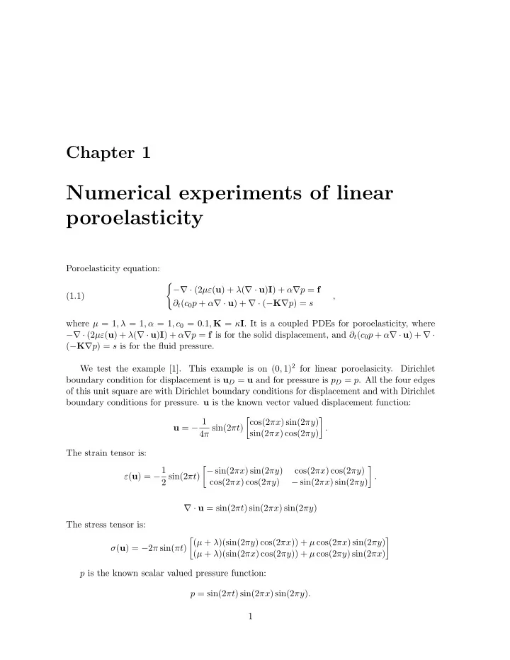
Chapter 1 Numerical experiments of linear poroelasticity Poroelasticity equation: � −∇ · (2 µε ( u ) + λ ( ∇ · u ) I ) + α ∇ p = f (1.1) , ∂ t ( c 0 p + α ∇ · u ) + ∇ · ( − K ∇ p ) = s where µ = 1 , λ = 1 , α = 1 , c 0 = 0 . 1 , K = κ I . It is a coupled PDEs for poroelasticity, where −∇ · (2 µε ( u ) + λ ( ∇ · u ) I ) + α ∇ p = f is for the solid displacement, and ∂ t ( c 0 p + α ∇ · u ) + ∇ · ( − K ∇ p ) = s is for the fluid pressure. This example is on (0 , 1) 2 for linear poroelasicity. We test the example [1]. Dirichlet boundary condition for displacement is u D = u and for pressure is p D = p . All the four edges of this unit square are with Dirichlet boundary conditions for displacement and with Dirichlet boundary conditions for pressure. u is the known vector valued displacement function: � cos(2 πx ) sin(2 πy ) � u = − 1 4 π sin(2 πt ) . sin(2 πx ) cos(2 πy ) The strain tensor is: ε ( u ) = − 1 � − sin(2 πx ) sin(2 πy ) � cos(2 πx ) cos(2 πy ) 2 sin(2 πt ) . cos(2 πx ) cos(2 πy ) − sin(2 πx ) sin(2 πy ) ∇ · u = sin(2 πt ) sin(2 πx ) sin(2 πy ) The stress tensor is: � ( µ + λ )(sin(2 πy ) cos(2 πx )) + µ cos(2 πx ) sin(2 πy ) � σ ( u ) = − 2 π sin( πt ) ( µ + λ )(sin(2 πx ) cos(2 πy )) + µ cos(2 πy ) sin(2 πx ) p is the known scalar valued pressure function: p = sin(2 πt ) sin(2 πx ) sin(2 πy ) . 1

2 CHAPTER 1. NUMERICAL EXPERIMENTS OF LINEAR POROELASTICITY � cos(2 πx ) sin(2 πy ) � ∇ p = 2 π sin(2 πt ) sin(2 πx ) cos(2 πy ) So right hand side of linear poroelasticity: � cos(2 πx ) sin(2 πy ) � f = ( − 2 µ − λ + α )2 π sin(2 πt ) , sin(2 πx ) cos(2 πy ) s = (sin(2 πx ) sin(2 πy ))(2 π cos(2 πt )( c 0 + α ) + 8 π 2 κ sin(2 πt )) . In Matlab code, we used the monolithic system, by matrix-concatenation. Numerical pressure elementwise at fime time Numerical displacement elementwise at final time 1 1 0.8 0.9 0.9 0.6 0.8 0.8 0.4 0.7 0.7 0.2 0.6 0.6 0.5 0 0.5 0.4 0.4 -0.2 0.3 0.3 -0.4 0.2 0.2 -0.6 0.1 0.1 -0.8 0 0 0 0.2 0.4 0.6 0.8 1 0 0.2 0.4 0.6 0.8 1 Figure 1.1: Left : Displacement with n = 32, κ = 10 − 6 . Right : Pressure with n = 32, κ = 10 − 6 . Numerical pressure elementwise at fime time Numerical displacement elementwise at final time 1 1 0.9 0.8 0.9 0.8 0.6 0.8 0.7 0.4 0.7 0.6 0.2 0.6 0.5 0 0.5 0.4 0.4 -0.2 0.3 0.3 -0.4 0.2 0.2 -0.6 0.1 0.1 -0.8 0 0 0 0.1 0.2 0.3 0.4 0.5 0.6 0.7 0.8 0.9 1 0 0.2 0.4 0.6 0.8 1 Figure 1.2: Left : Displacement with n = 32, κ = 1. Right : Pressure with n = 32, κ = 1. We have numerical tests [1] for κ = 1 , 10 − 3 , 10 − 6 , 10 3 using the monolithic system. Fol- lowing figures are numerical displacement and pressure based on different κ when n = 32.

3 Numerical pressure elementwise at fime time Numerical displacement elementwise at final time 1 1 0.9 0.8 0.9 0.8 0.6 0.8 0.7 0.4 0.7 0.6 0.2 0.6 0.5 0 0.5 0.4 0.4 -0.2 0.3 0.3 -0.4 0.2 0.2 -0.6 0.1 0.1 -0.8 0 0 0 0.2 0.4 0.6 0.8 1 0 0.2 0.4 0.6 0.8 1 Figure 1.3: Left : Displacement with n = 32, κ = 10 3 . Right : Pressure with n = 32, κ = 10 3 . Table 1.1: Errors of numerical value with different κ κ = 10 − 6 κ = 10 3 κ = 1 error max(ErrDsplT) max(ErrPresT) max(ErrDsplT) max(ErrPresT) max(ErrDsplT) max(ErrPresT) n = 16 2.6488E-03 2.4404E-01 8.1006E-03 1.6961E-02 8.3049E-03 1.2560E-02 n = 32 1.6019E-03 1.3404E-01 3.9255E-03 5.4317E-03 4.0192E-03 3.1964E-03 n = 128 8.6522E-04 7.0095E-02 1.9366E-03 1.9185E-03 1.9811E-03 8.0311E-04 Table 1.2: Convergence rates of errors in the numerical displacement with time steps,Q1, [1] n L2L2ErrDispl. conv. rate n = 8 2.1187E-03 – n = 16 6.8777E-04 1.6232 n = 32 2.6531E-04 1.3742 n = 64 1.1697E-04 1.1815 n = 128 5.5224E-05 1.0828 The table shows the maximum of differences of the exactly displacement and numerical displacement, and the maximum of differences of the exactly pressure and numerical pressure with n = 16 , 32 , 64, κ = 10 − 6 , 1 , 10 3 . [1] For calculating L2 error in space in one time step, find the difference between exact dis- placement u ( · , t n ) and the numerical value u ( n ) h ( · ) and then calculate the L2 error on the domain Ω. � 2 � � � u ( · , t n ) − u ( n ) h ( · ) , � � � Ω where t n means the time step. On the unit square domain, we have a mesh. And we calculate the L2 error on each element simultaneously. � 2 � � � u ( · , t n ) − u ( n ) � h ( · ) , � � � E E ∈ ε h where E means a element of the mesh, calculate the L2 error simultaneously on all the elements in the domain. In order to get the best numerical estimate of an integral, we pick Gaussian

4 CHAPTER 1. NUMERICAL EXPERIMENTS OF LINEAR POROELASTICITY quadrature points in each element. Nq 2 � � � u ( x k , y k , t n ) − u ( n ) � � w k h ( x k , y k ) | E | , � � � k =1 E ∈ ǫ h where N q is the number of Gaussian quadrature points on each element, w k is the weight of Gaussian quadrature points, ( x k , y k ) is the coordinates of Gaussian quadrature points correspond to each element, and | E | is the area of each element. So we can derive the formula to calculate the L2 error in space. For calculating L2 error in space and in all time steps, we name it as L2(L2)err, we need to take time division into consideration. We map the time section [0 , T ] to the Banach space, where it is a vector space with norm. So we can calculate the norm of L2 error in time. That is, if we have the mapping g, maps [0 , T ] to the Banach space, we derive the norm of g ( t ) is �� [0 ,T ] || g ( t ) | | 2 dt. Here, we have the same time step ∆ t with N T time steps totally. So the L2 error in displacement and time is � N T � � 2 � � � u ( · , t n ) − u ( n ) � � L2(L2)err = ∆ t n h ( · ) . � � � � Ω n =1 Another example [2] is on a square domain. Since the pressure occurs when the domain has low permeability for a short time interval, this example sets the final time as T = 10 − 3 . The value of permeability is κ = 10 − 6 . The Lam´ e coefficients are λ = 12500 and µ = 8333. On the top edge of the domain, p = 0, σ · n = (0 , − 1) t . The boundary conditions of other sides are: ∇ p · n = 0, u = 0 . The figure shows the numerical pressure at final time. From the Numerical pressure elementwise at final time 1 0.9 0.9 0.8 0.8 0.7 0.7 0.6 0.6 0.5 0.5 0.4 0.4 0.3 0.3 0.2 0.2 0.1 0.1 0 0 0.2 0.4 0.6 0.8 1 Figure 1.4: Left : Numerical Pressure with n = 40. Right : Contours of numerical pressure with n = 40. contour of the numerical pressure, we can see the pressure value.

Bibliography [1] Lorenz Berger, Rafel Bordas, David Kay, and Simon. Stabilized lowest-order finite element approximation for linear three-field poroelasticity. SIAM J. Sci. Comput. , 37:A2222– A2245, 2015. [2] Xiaozhe Hu, Carmen Rodrigo, Francisco J. Gaspar, and Ludmil Zikatanov. A nonconform- ing finite element method for the biot’s consolidation model in poroelasticity. J. Comput. Appl. Math. , 310:143–154, 2017. 5