
1 cs533d-winter-2005
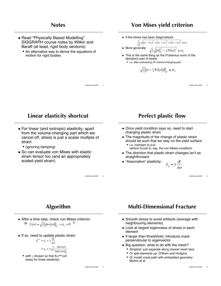
Notes
Read “Physically Based Modelling”
SIGGRAPH course notes by Witkin and Baraff (at least, rigid body sections)
- An alternative way to derive the equations of
motion for rigid bodies
2 cs533d-winter-2005
Von Mises yield criterion
If the stress has been diagonalized: More generally: This is the same thing as the Frobenius norm of the
deviatoric part of stress
- i.e. after subtracting off volume-changing part:
1 2 1 2
( )
2 + 2 3
( )
2 + 3 1
( )
2 Y
3 2
F
2 1 3 Tr
( )
2 Y
3 2 1 3 Tr
( )I F Y
3 cs533d-winter-2005
Linear elasticity shortcut
For linear (and isotropic) elasticity, apart
from the volume-changing part which we cancel off, stress is just a scalar multiple of strain
- (ignoring damping)
So can evaluate von Mises with elastic
strain tensor too (and an appropriately scaled yield strain)
4 cs533d-winter-2005
Perfect plastic flow
Once yield condition says so, need to start
changing plastic strain
The magnitude of the change of plastic strain
should be such that we stay on the yield surface
- I.e. maintain f()=0
(where f()0 is, say, the von Mises condition)
The direction that plastic strain changes isn’t as
straightforward
“Associative” plasticity:
˙
- p = f
- 5
cs533d-winter-2005
Algorithm
After a time step, check von Mises criterion:
is ?
If so, need to update plastic strain:
- with chosen so that f(new)=0
(easy for linear elasticity)
f () =
3 2 dev
( ) F Y > 0
p
new = p + f
- = p +
3 2
dev() dev() F
6 cs533d-winter-2005
Multi-Dimensional Fracture
Smooth stress to avoid artifacts (average with
neighbouring elements)
Look at largest eigenvalue of stress in each
element
If larger than threshhold, introduce crack
perpendicular to eigenvector
Big question: what to do with the mesh?
- Simplest: just separate along closest mesh face
- Or split elements up: O’Brien and Hodgins
- Or model crack path with embedded geometry:
Molino et al.