Notes Viscosity In reality, nearby molecules travelling at - PDF document

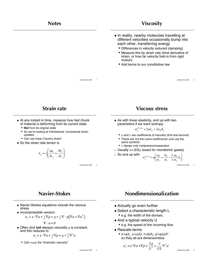
Notes Viscosity � In reality, nearby molecules travelling at different velocities occasionally bump into each other, transferring energy • Differences in velocity reduced (damping) • Measure this by strain rate (time derivative of strain, or how far velocity field is from rigid motion) • Add terms to our constitutive law cs533d-winter-2005 1 cs533d-winter-2005 2 Strain rate Viscous stress � At any instant in time, measure how fast chunk � As with linear elasticity, end up with two of material is deforming from its current state parameters if we want isotropy: • Not from its original state viscous = 2 µ ˙ ij + � ˙ � ij � � kk � ij • So we’re looking at infinitesimal, incremental strain • µ and � are coefficients of viscosity (first and second) updates • Can use linear Cauchy strain! • These are not the Lame coefficients! Just use the same symbols � So the strain rate tensor is • � damps only compression/expansion � � � Usually � � -2/3 µ (exact for monatomic gases) + � u j � u i ˙ ij = 1 � � � � � � So end up with � � 2 + � u j viscous = µ � u i � 2 � u k � x j � x i � � � ij � � ij � � � � x j � x i 3 � x k � � cs533d-winter-2005 3 cs533d-winter-2005 4 Navier-Stokes Nondimensionalization � Navier-Stokes equations include the viscous � Actually go even further stress � Select a characteristic length L � Incompressible version: • e.g. the width of the domain, ( ) � � � µ � u + � u T u t + u � � u + 1 � � p = g + 1 � And a typical velocity U � � u = 0 • e.g. the speed of the incoming flow � Often (but not always) viscosity µ is constant, � Rescale terms and this reduces to • x’=x/L, u’=u/U, t’=tU/L, p’=p/ � U 2 � � 2 u µ u t + u � � u + 1 � � p = g + so they all are dimensionless • Call � = µ / � the “kinematic viscosity” u ' t + u ' �� u ' + � p ' = Lg U 2 + � UL � 2 u ' cs533d-winter-2005 5 cs533d-winter-2005 6

Nondimensional parameters Why nondimensionalize? � Think of it as a user-interface issue � Re=UL/ � is the Reynold’s number � It lets you focus on what parameters matter • The smaller it is, the more viscosity plays a • If you scale your problem so nondimensional role in the flow parameters stay constant, solution scales • High Reynold’s numbers are hard to simulate � Code rot --- you may start off with code which has true dimensions, but as you hack around � Fr= is the Froude number U g L they lose meaning • The smaller it is, the more gravity plays a role • If you’re nondimensionalized, there should be only in the flow one or two parameters to play with • Note: often can ignore gravity (pressure � Not always the way to go --- you can look up material constants, but not e.g. Reynolds gradient cancels it out) numbers u t + u � � u + � p = (0, � 1,0) + 1 Re � 2 u Fr 2 cs533d-winter-2005 7 cs533d-winter-2005 8 Other quantities Boundary conditions � Inviscid flow: � We may want to carry around auxiliary • Solid wall: u•n=0 quantities • Free surface: p=0 (or atmospheric pressure) • E.g. temperature, the type of fluid (if we have • Moving solid wall: u•n=u wall •n a mix), concentration of smoke, etc. � Also enforced in-flow/out-flow • Between two fluids: u 1 •n=u 2 •n and p 1 =p 2 + �� � Use material derivative as before � Viscous flow: � E.g. if quantity doesn’t change, just is • No-slip wall: u=0 transported (“advected”) around: • Other boundaries can involve coupling tangential components of stress tensor… Dq Dt = q t + u � � q 3 = 0 � Pressure/velocity coupling at boundary: 1 2 • u•n modified by � p/ � n advection cs533d-winter-2005 9 cs533d-winter-2005 10 What now? Vorticity � Can solve numerically the full equations � How do we measure rotation? • Vorticity of a vector field (velocity) is: � = � � u • Will do this later • Proportional (but not equal) to angular velocity of a • Not so simple, could be expensive (3D) rigid body - off by a factor of 2 � Or make assumptions and simplify them, � Vorticity is what makes smoke look interesting then solve numerically • Turbulence • Simplify flow (e.g. irrotational) • Simplify dimensionality (e.g. go to 2D) cs533d-winter-2005 11 cs533d-winter-2005 12

Vorticity equation Vorticity equation continued � Start with N-S, constant viscosity and density � Simplify with more vector identities, and assume � � p = g + � � 2 u u t + u � � u + 1 incompressible to get: � Take curl of whole equation D � Dt = � � � u + � � 2 � � � p = � � g + � � � � 2 u ( ) � � u t + � � u � � u ( ) + � � 1 � Important result: Kelvin Circulation Theorem � Lots of terms are zero: • Roughly speaking: if � =0 initially, and there’s no • g is constant (or the potential of some field) viscosisty, � =0 forever after (following a chunk of • With constant density, pressure term too fluid) ) = � � � � 2 u � � u t + � � u � � u ( � If fluid starts off irrotational, it will stay that way � Then use vector identities to simplify… (in many circumstances) ) = � � 2 � � u ( ( ) � u + 1 2 � u 2 ( ) � � u t + � � � � u ) = � � 2 � � t + � � � � u ( cs533d-winter-2005 13 cs533d-winter-2005 14 Potential flow Potential in time � If velocity is irrotational: � What if we have a free surface? � Use vector identity u• � u=( �� u) � u+ � |u| 2 /2 � � u = 0 � Assume • Which it often is in simple laminar flow • incompressible ( � •u=0), inviscid, irrotational ( �� u=0) � Then there must be a stream function (potential) • constant density such that: • thus potential flow (u= �� , � 2 � =0) u = � � � Then momentum equation simplifies � Solve for incompressibility: (using G=-gy for gravitational potential) 2 + 1 ( ) � u + 1 u t + � � u 2 � u � � p = g � � � � = 0 2 + 1 � � t + 1 2 � u � � p = �� G � If u•n is known at boundary, we can solve it cs533d-winter-2005 15 cs533d-winter-2005 16 Bernoulli’s equation Water waves � Every term in the simplified momentum � For small waves (no breaking), can reduce geometry of water to 2D heightfield equation is a gradient: integrate to get 2 u 2 + p � Can reduce the physics to 2D also � t + 1 � = � G • How do surface waves propagate? � Plan of attack • (Remember Bernoulli’s law for pressure?) • Start with potential flow, Bernoulli’s equation � This tells us how the potential should • Write down boundary conditions at water surface evolve in time • Simplify 3D structure to 2D cs533d-winter-2005 17 cs533d-winter-2005 18

Set up Boundaries � y = 0 � We’ll take y=0 as the height of the water at � At sea floor (y=-H), v=0 rest � At sea surface (y=h � 0), v=h t � H is the depth (y=-H is the sea bottom) • Note again - assuming very small horizontal motion � h is the current height of the water at (x,z) � y = h t � Simplification: velocities very small (small amplitude waves) � At sea surface (y=h � 0), p=0 • Or atmospheric pressure, but we only care about pressure differences • Use Bernoulli’s equation, throw out small velocity squared term, use p=0, � t = � gh cs533d-winter-2005 19 cs533d-winter-2005 20 Finding a wave solution Dispersion relation � Plug in � =f(y)sin(K•(x,z)- � t) � So the wave speed c is • In other words, do a Fourier analysis in g c = � k tanh kH k = horizontal component, assume nothing much happens in vertical � Notice that waves of different wave- • Solving � 2 � =0 with boundary conditions on � y numbers k have different speeds gives ( ) cosh K ( y + H ) • Separate or disperse in time � = A � ( ) sin K � ( x , z ) � � t ( ) K sinh K H � For deep water (H big, k reasonable -- not tsunamis) tanh(kH) � 1 • Pressure boundary condition then gives (with k=|K|, the magnitude of K) g c = � = gk tanh kH k cs533d-winter-2005 21 cs533d-winter-2005 22 Simulating the ocean Energy spectrum � Far from land, a reasonable thing to do is � Fourier decomposition of height field: • Do Fourier decomposition of initial surface ˆ ( ) � x , z ( ) � � 1 i , j h ( x , z , t ) = h i , j , t ( ) e height i , j 2 • Evolve each wave according to given wave S ( K ) = ˆ � “Energy” in K=(i,j) is h ( K ) speed (dispersion relation) � Update phase, use FFT to evaluate � Oceanographic measurements have found � How do we get the initial spectrum? models for expected value of S(K) • Measure it! (oceanography) (statistical description) cs533d-winter-2005 23 cs533d-winter-2005 24