Neurons (nerve cells) Faculty of Science The stochastic - - PowerPoint PPT Presentation

u n i v e r s i t y o f c o p e n h a g e n

Faculty of Science

The stochastic Morris-Lecar neuron model embeds a one-dimensional diffusion and its first-passage-time crossings

Aarhus, 2013 Susanne Ditlevsen Cindy Greenwood Patrick Jahn Rune Berg

April, 2013 Slide 1/30

u n i v e r s i t y o f c o p e n h a g e n d e p a r t m e n t o f m a t h e m a t i c a l s c i e n c e s

Neurons (nerve cells)

= ⇒

• Slide 2/30— Susanne Ditlevsen — The stochastic Morris-Lecar neuron model embeds a one-dimensional diffusion and its first-passage-time crossings — April, 2013

u n i v e r s i t y o f c o p e n h a g e n d e p a r t m e n t o f m a t h e m a t i c a l s c i e n c e s

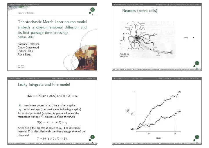
Leaky Integrate-and-Fire model

dXt = µ(Xt) dt + σ(Xt) dW (t) ; X0 = x0 Xt: membrane potential at time t after a spike x0: initial voltage (the reset value following a spike) An action potential (a spike) is produced when the membrane voltage Xt exceeds a firing threshold S(t) = S > X(0) = x0 After firing the process is reset to x0. The interspike interval T is identified with the first-passage time of the threshold, T = inf{t > 0 : Xt ≥ S}.

Slide 3/30— Susanne Ditlevsen — The stochastic Morris-Lecar neuron model embeds a one-dimensional diffusion and its first-passage-time crossings — April, 2013

u n i v e r s i t y o f c o p e n h a g e n d e p a r t m e n t o f m a t h e m a t i c a l s c i e n c e s

time X(t) T T S x0

Slide 4/30— Susanne Ditlevsen — The stochastic Morris-Lecar neuron model embeds a one-dimensional diffusion and its first-passage-time crossings — April, 2013

u n i v e r s i t y o f c o p e n h a g e n d e p a r t m e n t o f m a t h e m a t i c a l s c i e n c e s

Two commonly used Leaky Integrate-and-Fire neuron models (I)

The Ornstein-Uhlenbeck process: dXt =

• −Xt

τ + µ

• dt + σ dWt ; X0 = x0.

where Xt: membrane potential at time t after a spike τ: membrane time constant, reflects spontaneous voltage decay (> 0) µ: characterizes constant neuronal input σ: characterizes erratic neuronal input x0: initial voltage (the reset value following a spike)

Slide 5/30— Susanne Ditlevsen — The stochastic Morris-Lecar neuron model embeds a one-dimensional diffusion and its first-passage-time crossings — April, 2013

u n i v e r s i t y o f c o p e n h a g e n d e p a r t m e n t o f m a t h e m a t i c a l s c i e n c e s

Two commonly used Leaky Integrate-and-Fire neuron models (II)

The Feller process (also CIR or square root process): d(Xt − VI) =

• −Xt − VI

τ + µ

• dt + σ
• Xt − VI dWt;

X0 = x0 ≥ VI. where VI: inhibitory reversal potential and 2µ ≥ σ2

Slide 6/30— Susanne Ditlevsen — The stochastic Morris-Lecar neuron model embeds a one-dimensional diffusion and its first-passage-time crossings — April, 2013

u n i v e r s i t y o f c o p e n h a g e n d e p a r t m e n t o f m a t h e m a t i c a l s c i e n c e s

Intracellular recording of membrane potential

time (ms)

−50 500

measured membrane voltage, V(t)

Slide 7/30— Susanne Ditlevsen — The stochastic Morris-Lecar neuron model embeds a one-dimensional diffusion and its first-passage-time crossings — April, 2013

u n i v e r s i t y o f c o p e n h a g e n d e p a r t m e n t o f m a t h e m a t i c a l s c i e n c e s

Spike generation

time (ms) standard deviation

−10 −5 5 10 1 2 3 4 5 6 7

(b)

Slide 8/30— Susanne Ditlevsen — The stochastic Morris-Lecar neuron model embeds a one-dimensional diffusion and its first-passage-time crossings — April, 2013

u n i v e r s i t y o f c o p e n h a g e n d e p a r t m e n t o f m a t h e m a t i c a l s c i e n c e s

Spike generation

A Global Jump Diffusion Model dXt = 1 τ(Xt)(a+g(t)−Xt)dt+σ(Xt)dWt+(x∗−Xt−)µ(Xt−, dt), where µ(Xt−, dt) is a Poisson random measure with intensity measure λ(Xt−)dt. Estimator: ˆ λ(x) := l

j=1 1[x− h

2 ,x+ h 2 ](Ysj)

M

i=1 ∆1[x− h

2 ,x+ h 2 ](Yi)

,

Slide 9/30— Susanne Ditlevsen — The stochastic Morris-Lecar neuron model embeds a one-dimensional diffusion and its first-passage-time crossings — April, 2013

u n i v e r s i t y o f c o p e n h a g e n d e p a r t m e n t o f m a t h e m a t i c a l s c i e n c e s

Estimation of spike intensity

• x (mV)

λ λ (

(1 ms) )

(a)

−55 −50 −45 0.1 0.2

• x (mV)

log(

(λ

λ)

)

(b)

−55 −50 −45 −7 −6 −5 −4 −3 −2

Final estimate: ˆ λ(x) = exp (15.3 + 0.4x) = exp x − (−38.25) 2.5

• Slide 10/30— Susanne Ditlevsen — The stochastic Morris-Lecar neuron model embeds a one-dimensional diffusion and its first-passage-time crossings — April, 2013

u n i v e r s i t y o f c o p e n h a g e n d e p a r t m e n t o f m a t h e m a t i c a l s c i e n c e s

time (s)

20 mV

9.0 9.1 9.2 9.3 9.4 9.5

data model

Slide 11/30— Susanne Ditlevsen — The stochastic Morris-Lecar neuron model embeds a one-dimensional diffusion and its first-passage-time crossings — April, 2013

u n i v e r s i t y o f c o p e n h a g e n d e p a r t m e n t o f m a t h e m a t i c a l s c i e n c e s

The Morris Lecar model

dVt = 1 C (−gCam∞(Vt)(Vt − VCa) − gKWt(Vt − VK) −gL(Vt − VL) + I)dt dWt = (α(Vt)(1 − Wt) − β(Vt)Wt) dt with the auxiliary functions given by m∞(v) = 1 2

• 1 + tanh

v − V1 V2

• α(v)

= 1 2φ cosh v − V3 2V4 1 + tanh v − V3 V4

• β(v)

= 1 2φ cosh v − V3 2V4 1 − tanh v − V3 V4

• Slide 12/30— Susanne Ditlevsen — The stochastic Morris-Lecar neuron model embeds a one-dimensional diffusion and its first-passage-time crossings — April, 2013

u n i v e r s i t y o f c o p e n h a g e n d e p a r t m e n t o f m a t h e m a t i c a l s c i e n c e s

200 400 600 800 1000 −40 −20 20 time membrane voltage, V(t)

Slide 13/30— Susanne Ditlevsen — The stochastic Morris-Lecar neuron model embeds a one-dimensional diffusion and its first-passage-time crossings — April, 2013

u n i v e r s i t y o f c o p e n h a g e n d e p a r t m e n t o f m a t h e m a t i c a l s c i e n c e s

−40 −20 20 40 0.1 0.2 0.3 0.4 0.5 membrane voltage Vt normalized conductance Wt

• (A)

Slide 14/30— Susanne Ditlevsen — The stochastic Morris-Lecar neuron model embeds a one-dimensional diffusion and its first-passage-time crossings — April, 2013

u n i v e r s i t y o f c o p e n h a g e n d e p a r t m e n t o f m a t h e m a t i c a l s c i e n c e s

The stochastic Morris Lecar model

dVt = 1 C (−gCam∞(Vt)(Vt − VCa) − gKWt(Vt − VK) −gL(Vt − VL) + I)dt dWt = (α(Vt)(1 − Wt) − β(Vt)Wt) dt +σ

• 2 α(Vt)β(Vt)

α(Vt) + β(Vt)Wt(1 − Wt)dBt

Slide 15/30— Susanne Ditlevsen — The stochastic Morris-Lecar neuron model embeds a one-dimensional diffusion and its first-passage-time crossings — April, 2013

u n i v e r s i t y o f c o p e n h a g e n d e p a r t m e n t o f m a t h e m a t i c a l s c i e n c e s

−40 −20 20 40 0.1 0.2 0.3 0.4 0.5 membrane voltage, V(t) normalized conductance, W(t)

• Slide 16/30— Susanne Ditlevsen — The stochastic Morris-Lecar neuron model embeds a one-dimensional diffusion and its first-passage-time crossings — April, 2013

u n i v e r s i t y o f c o p e n h a g e n d e p a r t m e n t o f m a t h e m a t i c a l s c i e n c e s

time

−50 2000 4000

membrane voltage, V(t)

0.2 0.4

normalized conductance, W(t) time

−50 2000 4000

membrane voltage, V(t)

0.2 0.4

normalized conductance, W(t)

σ = 0.2 σ = 0.5

Slide 17/30— Susanne Ditlevsen — The stochastic Morris-Lecar neuron model embeds a one-dimensional diffusion and its first-passage-time crossings — April, 2013

u n i v e r s i t y o f c o p e n h a g e n d e p a r t m e n t o f m a t h e m a t i c a l s c i e n c e s

Linearization around the equilibrium point

Xt = Vt − Veq Wt − Weq

• Small noise: the dynamics concentrate around the

equilibrium point x = (0, 0). Linear approximation: dXt ≈ MXtdt + GdBt where M =

• ∂f ∗

∂x ∂f ∗ ∂y ∂g∗ ∂x ∂g∗ ∂y

• x=(0,0)

=

• 0.026

−22.96 0.00034 −0.045

• Slide 18/30— Susanne Ditlevsen — The stochastic Morris-Lecar neuron model embeds a one-dimensional diffusion and its first-passage-time crossings — April, 2013

u n i v e r s i t y o f c o p e n h a g e n d e p a r t m e n t o f m a t h e m a t i c a l s c i e n c e s

Deterministic approximation

Xt ≈ C cos ωt sin ωt

• e−λt

where C = x0 (m2y0 + (m1 + λ)x0)/ω y0 (m3x0 − (m1 + λ)y0)/ω

• .

and −λ ± ωi = −0.0094 ± 0.0803i are the eigenvalues of M. Note typical time scales of the system: λt and ωt and λ ≪ ω.

Slide 19/30— Susanne Ditlevsen — The stochastic Morris-Lecar neuron model embeds a one-dimensional diffusion and its first-passage-time crossings — April, 2013

u n i v e r s i t y o f c o p e n h a g e n d e p a r t m e n t o f m a t h e m a t i c a l s c i e n c e s

Deterministic approximation

time

−30 −25 500 1000

membrane voltage, V(t)

0.12 0.14

normalized conductance, W(t) exact approx

Slide 20/30— Susanne Ditlevsen — The stochastic Morris-Lecar neuron model embeds a one-dimensional diffusion and its first-passage-time crossings — April, 2013

u n i v e r s i t y o f c o p e n h a g e n d e p a r t m e n t o f m a t h e m a t i c a l s c i e n c e s

Clarifying transformations

If dXt = MXtdt + GdBt then Xt = QR−ωt τ √ λ Uλt = τ √ λ −ω m1 + λ m3 cos ωt sin ωt − sin ωt cos ωt

• Uλt

where dUt = −Utdt + 1 τ Rωt/λCd ˜ Bt.

Slide 21/30— Susanne Ditlevsen — The stochastic Morris-Lecar neuron model embeds a one-dimensional diffusion and its first-passage-time crossings — April, 2013

u n i v e r s i t y o f c o p e n h a g e n d e p a r t m e n t o f m a t h e m a t i c a l s c i e n c e s

Stochastic approximation

Theorem (Baxendale and Greenwood)

For each fixed t∗ > 0 and x ∈ I R2 Ut

D

− → St as λ/ω → 0 where {St : 0 ≤ t ≤ t∗} is the standardized two-dimensional OU process generated by dSt = −Stdt + dBt with U0 = S0 = x. Thus, √ λ τ Q−1Xt ≈ cos ωt sin ωt − sin ωt cos ωt

• Sλt

Slide 22/30— Susanne Ditlevsen — The stochastic Morris-Lecar neuron model embeds a one-dimensional diffusion and its first-passage-time crossings — April, 2013

u n i v e r s i t y o f c o p e n h a g e n d e p a r t m e n t o f m a t h e m a t i c a l s c i e n c e s

Firing in the approximate model

√ λ τ Q−1Xt ≈ cos ωt sin ωt − sin ωt cos ωt

• Sλt

For fixed t the transformed solution √ λQ−1Xt/τ is the counterclockwise rotation of angle ωt of the orthogonal pair (S(1)

λt , S(2) λt ).

Transformed space: ˜ V ˜ W

• =

√ λ τ Q−1 V − Veq W − Weq

• Slide 23/30— Susanne Ditlevsen — The stochastic Morris-Lecar neuron model embeds a one-dimensional diffusion and its first-passage-time crossings — April, 2013

u n i v e r s i t y o f c o p e n h a g e n d e p a r t m e n t o f m a t h e m a t i c a l s c i e n c e s

Firing in the approximate model

Modulus of Sλt is a radial OU process: Zλt =

• (S(1)

λt )2 + (S(2) λt )2

It solves dZλt = 1 2Zλt − Zλt

• dt + dWλt

Firing could then be identified with T = inf{t > 0 : Zλt ≥ z} How to choose z?

Slide 24/30— Susanne Ditlevsen — The stochastic Morris-Lecar neuron model embeds a one-dimensional diffusion and its first-passage-time crossings — April, 2013

u n i v e r s i t y o f c o p e n h a g e n d e p a r t m e n t o f m a t h e m a t i c a l s c i e n c e s

Reconstructing the stochastic ML firing mechanism

−35 −30 −25 −20 −15 −10 −5 0.10 0.12 0.14 0.16 0.18 0.20 membrane voltage Vt normalized conductance Wt

• Slide 25/30— Susanne Ditlevsen — The stochastic Morris-Lecar neuron model embeds a one-dimensional diffusion and its first-passage-time crossings — April, 2013

u n i v e r s i t y o f c o p e n h a g e n d e p a r t m e n t o f m a t h e m a t i c a l s c i e n c e s

Probability of firing

• ● ● ● ● ● ● ● ● ● ● ●
• ● ● ● ● ●

0.005 0.015 0.025 0.0 0.2 0.4 0.6 0.8 1.0 distance from fixed point conditional probability of firing

(A)

1 2 3 4 0.0 0.2 0.4 0.6 0.8 1.0 distance in transformed space conditional probability of firing

(B)

Original space Transformed space p(l) = 1 1 + exp((α − l)/β) p(r) = 1 1 + exp((α∗ − r)/β∗) where α∗ = α √ 2λ/σ

Slide 26/30— Susanne Ditlevsen — The stochastic Morris-Lecar neuron model embeds a one-dimensional diffusion and its first-passage-time crossings — April, 2013

u n i v e r s i t y o f c o p e n h a g e n d e p a r t m e n t o f m a t h e m a t i c a l s c i e n c e s

The density of the interspike interval T

Conditional hazard rate: α(t, r) = lim

∆t→0

1 ∆t P(t ≤ T < t + ∆t | T ≥ t, Zλt = r). Unconditional distribution: P(T > t) = E

• exp
• −

t α(Zλs)ds

• On average, the process crosses L every 2π/ω = 78.2

time units. Estimated hazard rate: α(t, r) = α(r) = ω 2π 1 1 + exp((α∗ − r)/β∗). Note that it is bounded. (Is it realistic? Refractory period?)

Slide 27/30— Susanne Ditlevsen — The stochastic Morris-Lecar neuron model embeds a one-dimensional diffusion and its first-passage-time crossings — April, 2013

u n i v e r s i t y o f c o p e n h a g e n d e p a r t m e n t o f m a t h e m a t i c a l s c i e n c e s

Final model

dZu = 1 2Zu − Zu

• dt + dWu − Zu−µ(Zu−, du),

where µ(Zu−, du) is a Poisson measure with intensity α(Zu−), and Zu− denotes the left limit of Zu. Other possible hazard rates: From turtle motoneuron data: α(r) = exp((r − α)/β) Hard threshold (standard LIF model): α(r) = δS(r) where S is the threshold. How to choose S?

Slide 28/30— Susanne Ditlevsen — The stochastic Morris-Lecar neuron model embeds a one-dimensional diffusion and its first-passage-time crossings — April, 2013

u n i v e r s i t y o f c o p e n h a g e n d e p a r t m e n t o f m a t h e m a t i c a l s c i e n c e s ISI distribution 500 1000 1500 2000 0.001 0.002

Black line: Sigmoidal hazard rate Gray line: Exponential haxard rate Dashed line: Hard threshold, S chosen such that E(T) = S2

2 2F2 (1, 1; 2, 2; S2) coincides with the simulated

data (threshold is lower than the unstable limit cycle).

Slide 29/30— Susanne Ditlevsen — The stochastic Morris-Lecar neuron model embeds a one-dimensional diffusion and its first-passage-time crossings — April, 2013

u n i v e r s i t y o f c o p e n h a g e n d e p a r t m e n t o f m a t h e m a t i c a l s c i e n c e s

References

Berg, R. W., Alaburda, A., and Hounsgaard, J. (2007). Balanced inhibition and excitation drive spike activity in spinal halfcenters. Science, 315, 390–393. Berg, R. W., Ditlevsen, S., and Hounsgaard, J. (2008). Intense synaptic activity enhances temporal resolution in spinal motoneurons. PLoS ONE, 3, e3218. Ditlevsen, S. and Greenwood, P. (2012). The Morris-Lecar neuron model embeds a leaky integrate-and-fire model. To appear in J. Math. Biol. DOI: 10.1007/s00285-012-0552-7. Jahn, P., Berg, R. W., Hounsgaard, J., and Ditlevsen, S. (2011). Motoneuron membrane potentials follow a time inhomogeneous jump diffusion process. J. Comp. Neurosci., 31, 563–579.

Slide 30/30— Susanne Ditlevsen — The stochastic Morris-Lecar neuron model embeds a one-dimensional diffusion and its first-passage-time crossings — April, 2013