cs 403 path planning
play

CS 403 - Path Planning Roderic A. Grupen 4/2/19 Robotics 1 - PowerPoint PPT Presentation

Why Motion Planning? CS 403 - Path Planning Roderic A. Grupen 4/2/19 Robotics 1 4/2/19 Robotics 2 Why Motion Planning? Summary GE Control Virtual Prototyping Character Animation Kinematics Structural Molecular Biology


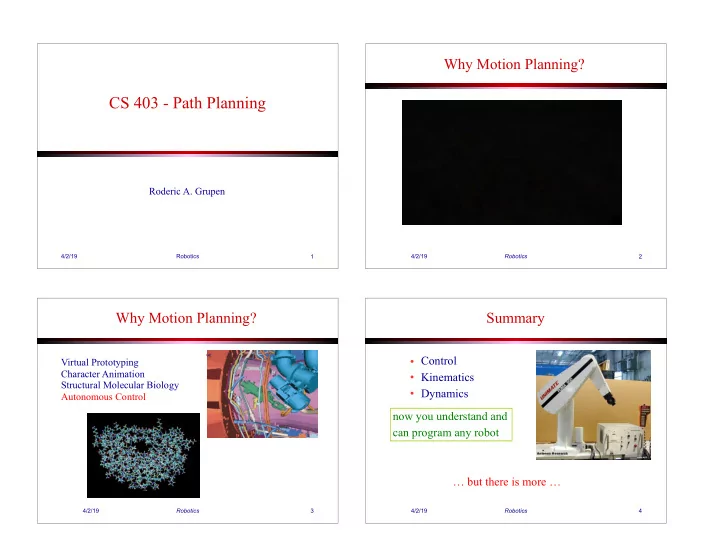
  1. Why Motion Planning? CS 403 - Path Planning Roderic A. Grupen 4/2/19 Robotics � 1 4/2/19 Robotics � 2 Why Motion Planning? Summary GE • Control Virtual Prototyping Character Animation • Kinematics Structural Molecular Biology • Dynamics Autonomous Control now you understand and can program any robot … but there is more … 4/2/19 Robotics � 3 4/2/19 Robotics � 4

  2. C-Space Construction for n DOF Origins of Motion Planning • 6 revolute degrees of freedom (e.g. Puma) • T. Lozano-Pérez and M.A. Wesley: 
 • 2 p range of motion per joint “An Algorithm for Planning Collision-Free Paths Among • 2 x 10 15 configurations Polyhedral Obstacles,” 1979. • 1 million checks per second • 69 years of computation • introduced the notion of configuration space (c-space) to robotics • many approaches have been devised since then in configuration space naïve grid method is impossible 4/2/19 Robotics � 5 4/2/19 Robotics � 6 Representation Completeness of Planning Algorithms …given a moving object, A, initially in an unoccupied region of freespace, s, a set of stationary objects, B i , at known locations, and a goal position, g, … a complete planner finds a path if one exists resolution complete – complete to the model resolution find a sequence of collision-free motions that take A from s to g probabilistically complete 4/2/19 Robotics � 7 4/2/19 Robotics � 8

  3. Sliding Along the Boundary Computing C-Space: Growing Obstacles Workspace Configuration Space How about changing θ ? � 9 � 10 Translational Case (fixed orientation) Obstacles in 3D (x,y, q ) Obstacle Robot C-Space Obstacle Reference Point � 11 4/2/19 Robotics � 12 Jean-Claude Latombe

  4. Exact Cell Decomposition Exact Cell Decomposition Jean-Claude Latombe 4/2/19 Robotics � 13 4/2/19 Robotics � 14 Exact Cell Decomposition Representation – Simplicial Decomposition Schwartz and Sharir Lozano-Perez Canny 4/2/19 Robotics � 15 4/2/19 Robotics � 16 Jean-Claude Latombe

  5. Approximate Methods: 2 n -Tree Approximate Cell Decomposition again…build a graph and search it to find a path 4/2/19 Robotics � 17 4/2/19 Robotics � 18 Jean-Claude Latombe Roadmap Representations Representation – Roadmaps Voronoi diagrams Visibility diagrams: a “retraction” unsmooth …the continuous freespace sensitive to error is represented as a network of curves… 4/2/19 Robotics � 19 4/2/19 Robotics � 20 Jean-Claude Latombe

  6. Summary Attractive Potential Fields • Exact Cell Decomposition + • Approximate Cell Decomposition • graph search • next: potential field methods • Roadmap Methods • visibility graphs - • Voronoi diagrams • next: probabilistic road maps (PRM) 4/2/19 Robotics � 21 � 22 Repulsive Potentials Electrostatic (or Gravitational) Field + - - depends on direction � 23 � 24

  7. Attractive Potential A Repulsive Potential rep ( q ) = 1 F x φ att ( q ) = 1 k ( q − q ref ) T ( q − q ref ) 2 att ( q ) = −∇φ att ( q ) F rep ( q ) = 1 − 1 F = − k ( q − q ref ) x δ 0 � 25 � 26 Repulsive Potential Sum Attractive and Repulsive Fields 2 ⎛ ⎞ ( q − q obst ) − 1 1 φ rep ( q ) = k if (( q − q obs ) < δ 0 ⎜ ⎟ ⎜ ⎟ δ 0 ⎝ ⎠ = 0 otherwise F rep ( q ) = −∇φ ( q ) ⎧ ⎫ ⎛ ⎞ ( q − q obs ) − 1 1 if (( q − q obs ) < δ 0 = − k ⎪ ⎜ ⎟ ⎪ ⎜ ⎟ ⎨ δ 0 ⎬ ⎝ ⎠ ⎪ ⎪ 0 otherwise ⎩ ⎭ 4/2/19 Robotics � 27 � 28

  8. Artificial Potential Function Potential Fields • Goal: avoid local minima φ att ( q ) φ rep ( q ) φ total ( q ) + = • Problem: requires global information = • Solution: Navigation Function + F rep F rep Robot F att total ( q ) = −∇φ total F F att Obstacle Goal � 29 4/2/19 Robotics � 30 Navigation Functions Navigation Functions Morse - Critical points are places where the gradient of φ vanishes, i.e. minima, saddle points, or maxima are called critical values. Navigation functions have no degenerate critical points where the Analyticity – navigation functions are analytic because they are robot can get stuck short of attaining the goal. infinitely differentiable and their Taylor series converge to φ (q 0 ) as q approaches q 0 Polar – gradients (streamlines) of navigation functions terminate at a unique minima Admissibility - practical potential fields must always generate bounded torques 4/2/19 Robotics � 31 4/2/19 Robotics � 32

  9. The Hessian Harmonic Functions multivariable control function, f(q 0 ,q 1 ,...,q n ) if the trace of the Hessian (the Laplacian) is 0 then function f is a harmonic function laminar fluid flow, steady state temperature distribution, if the Hessian is positive semi-definite over electromagnetic fields, current flow in conductive media the domain Q, then the function f is convex over Q 4/2/19 Robotics � 33 4/2/19 Robotics � 34 Properties of Harmonic Functions Properties of Harmonic Functions Min-Max Property - Mean-Value - up to truncation error, the value of the harmonic potential at a point in a lattice is the average of the ...in any compact neighborhood of freespace, the values of its 2n Manhattan neighbors. minimum and maximum of the function must occur on the boundary. ¼ ¼ ¼ analog & numerical methods ¼ 4/2/19 Robotics � 35 4/2/19 Robotics � 36

  10. Numerical Relaxation Harmonic Relaxation: Numerical Methods Gauss-Seidel Jacobi iteration Successive Over Relaxation 4/2/19 Robotics � 37 4/2/19 Robotics � 38 Properties of Harmonic Functions Minima in Harmonic Functions for some i, if ∂ 2 φ / ∂ x i2 > 0 (concave upward), then there must exist another dimension, j, where Hitting Probabilities - if we denote p(x) at state x as ∂ 2 φ / ∂ x j2 < 0 to satisfy Laplace’s constraint. the probability that starting from x, a random walk process will reach an obstacle before it reaches a goal—p(x) is known as the hitting probability greedy descent on the harmonic function minimizes the hitting probability. therefore, if you’re not at a goal, there is always a way downhill... ...there are no local minima... 4/2/19 Robotics � 39 4/2/19 Robotics � 40

  11. Configuration Space Harmonic Functions for Path Planning 4/2/19 Robotics � 41 4/2/19 Robotics � 42 Harmonic Functions for Path Planning Harmonic Functions for Path Planning 4/2/19 Robotics � 43 4/2/19 Robotics � 44

  12. Reactive Admittance Control ok, back to graphical methods… 4/2/19 Robotics � 45 4/2/19 Robotics � 46 Probabilistic Roadmaps (PRM) Probabilistic Roadmaps (PRM) • Construction • Generate random configurations • Eliminate if they are in collision • Use local planner to connect configurations • Expansion • Identify connected components • Resample gaps • Try to connect components • Query • Connect initial and final configuration to roadmap • Perform graph search 4/2/19 Robotics � 47 4/2/19 Robotics � 48

  13. Sampling Phase Complexity of Collision Detection • Construction • n objects have O(n 2 ) interactions – R = (V,E) • each object has perhaps thousands of features – repeat n times: • robot with l links and k obstacles has O(l k) – generate random configuration – add to V if collision free very costly – attempt to connect to neighbors using local planner, unless in same connected component of R 4/2/19 Robotics � 49 4/2/19 Robotics � 50 Local Planner Path Extraction • Connect start and goal configuration to roadmap using local planner q 2 • Perform graph search on roadmap • Computational cost of querying negligible compared to δ construction of roadmap q 1 tests up to a specified resolution δ ! 4/2/19 Robotics � 51 4/2/19 Robotics � 52

  14. Another Local Planner Another Look at the Sampling Phase • Construction – R = (V,E) – repeat n times: – generate random configuration – add to V if collision free – attempt to connect to neighbors using local planner , unless in same connected component of R • Expansion – repeat k times: – select difficult node perform random walk of predetermined length; – attempt to connect to neighbors using another local choose new direction randomly after hitting obstacle; planner attempt to connect to roadmap after random walk 4/2/19 Robotics � 53 4/2/19 Robotics � 54 Difficult Summary: PRM • Possible measures for difficulty of a • Algorithmically very simple configuration (vertex in R): • Surprisingly efficient even in high-dimensional C- spaces • 1/(# of nodes within given distance) • Capable of addressing a wide variety of motion • 1/distance to closest connected components planning problems • # of failures of local planner to connect to • One of the hottest areas of research neighbors • Allows probabilistic performance guarantees 4/2/19 Robotics � 55 4/2/19 Robotics � 56

  15. Variations of the PRM Lazy PRM observation: pre-computation of roadmap takes a long • Lazy PRMs time and does not respond well in dynamic • Rapidly-exploring Random Trees environments 4/2/19 Robotics � 57 4/2/19 Robotics � 58 Lazy PRM Lazy PRM • Incremental roadmap computation • Individual query slower than query with PRM • pre-computation eliminated • minimize number of distance computations • controllable computational expense 4/2/19 Robotics � 59 4/2/19 Robotics � 60

Download Presentation
Download Policy: The content available on the website is offered to you 'AS IS' for your personal information and use only. It cannot be commercialized, licensed, or distributed on other websites without prior consent from the author. To download a presentation, simply click this link. If you encounter any difficulties during the download process, it's possible that the publisher has removed the file from their server.

Recommend


More recommend