Network/Graph Network/Graph Informally a graph is a set of nodes - - PDF document

Network/Graph Network/Graph Theory Theory

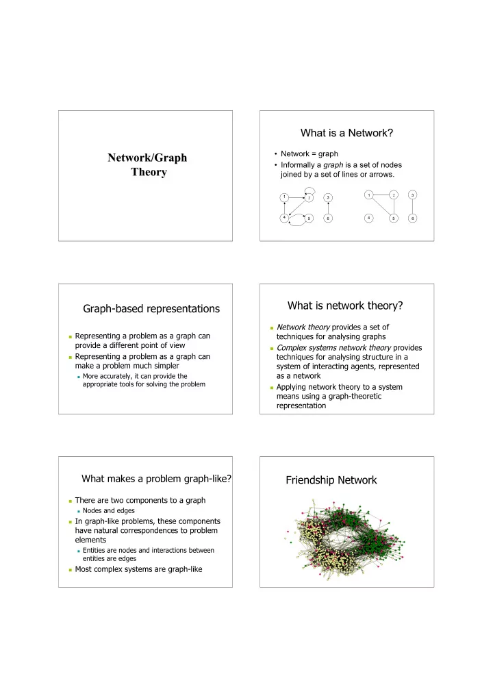
What is a Network? What is a Network?

• Network = graph
• Informally a graph is a set of nodes

joined by a set of lines or arrows.

1 1 2 3 4 4 5 5 6 6 2 3

Graph-based representations

 Representing a problem as a graph can

provide a different point of view

 Representing a problem as a graph can

make a problem much simpler

 More accurately, it can provide the

appropriate tools for solving the problem

What is network theory?

 Network theory provides a set of

techniques for analysing graphs

 Complex systems network theory provides

techniques for analysing structure in a system of interacting agents, represented as a network

 Applying network theory to a system

means using a graph-theoretic representation

What makes a problem graph-like?

 There are two components to a graph

 Nodes and edges

 In graph-like problems, these components

have natural correspondences to problem elements

 Entities are nodes and interactions between

entities are edges

 Most complex systems are graph-like

Friendship Network

Scientific collaboration network

Business ties in US biotech- industry

Genetic interaction network Protein-Protein Interaction Networks Transportation Networks Internet

Ecological Networks Graph Theory - History Graph Theory - History

Leonhard Euler's paper

• n “Seven Bridges of

Königsberg” , published in 1736.

Graph Theory - History Graph Theory - History

Cycles in Polyhedra Thomas P. Kirkman William R. Hamilton Hamiltonian cycles in Platonic graphs

Graph Theory - History Graph Theory - History

Gustav Kirchhoff Trees in Electric Circuits

Graph Theory - History Graph Theory - History

Arthur Cayley James J. Sylvester George Polya Enumeration of Chemical Isomers

Graph Theory - History Graph Theory - History

Francis Guthrie Auguste DeMorgan Four Colors of Maps

Definition: Graph Definition: Graph

• G is an ordered triple G:=(V, E, f)

– V is a set of nodes, points, or vertices. – E is a set, whose elements are known as edges or lines. – f is a function

• maps each element of E
• to an unordered pair of vertices in V.

Definitions Definitions

• Vertex

– Basic Element – Drawn as a node or a dot. – Vertex set of G is usually denoted by V(G), or V

• Edge

– A set of two elements – Drawn as a line connecting two vertices, called end vertices, or endpoints. – The edge set of G is usually denoted by E(G), or E.

Example

• V:={1,2,3,4,5,6}
• E:={{1,2},{1,5},{2,3},{2,5},{3,4},{4,5},{4,6}}

Simple Graphs

Simple graphs are graphs without multiple edges or self-loops.

Directed Graph (digraph) Directed Graph (digraph)

• Edges have directions

– An edge is an ordered pair of nodes

loop node multiple arc arc

Weighted graphs

1 2 3 4 5 6 .5 1.2 .2 .5 1.5 .3 1 4 5 6 2 3 2 1 3 5

• is a graph for which each edge has an

associated weight, usually given by a weight function w: E → R.

Structures and structural metrics

 Graph structures are used to isolate

interesting or important sections of a graph

 Structural metrics provide a measurement

• f a structural property of a graph

 Global metrics refer to a whole graph  Local metrics refer to a single node in a graph

Graph structures

 Identify interesting sections of a graph

 Interesting because they form a significant

domain-specific structure, or because they significantly contribute to graph properties

 A subset of the nodes and edges in a

graph that possess certain characteristics,

• r relate to each other in particular ways

Connectivity

• a graph is connected if

– you can get from any node to any other by following a sequence of edges OR – any two nodes are connected by a path.

• A directed graph is strongly connected if

there is a directed path from any node to any

• ther node.

Component Component

• Every disconnected graph can be split

up into a number of connected components.

Degree Degree

• Number of edges incident on a node

The degree of 5 is 3

Degree (Directed Graphs) Degree (Directed Graphs)

• In-degree: Number of edges entering
• Out-degree: Number of edges leaving
• Degree = indeg + outdeg
• utdeg(1)=2

indeg(1)=0

• utdeg(2)=2

indeg(2)=2

• utdeg(3)=1

indeg(3)=4

Degree: Simple Facts

• If G is a graph with m edges, then

Σ deg(v) = 2m = 2 |E |

• If G is a digraph then

Σ indeg(v)=Σ outdeg(v) = |E |

• Number of Odd degree Nodes is even

Walks

A walk of length k in a graph is a succession of k (not necessarily different) edges of the form uv,vw,wx,…,yz. This walk is denote by uvwx…xz, and is referred to as a walk between u and z. A walk is closed is u=z.

Path Path

• A path is a walk in which all the edges and all

the nodes are different.

Walks and Paths 1,2,5,2,3,4 1,2,5,2,3,2,1 1,2,3,4,6 walk of length 5 CW of length 6 path of length 4

Cycle

• A cycle is a closed path in which all the

edges are different.

1,2,5,1 2,3,4,5,2 3-cycle 4-cycle

Special Types of Graphs

• Empty Graph / Edgeless graph

– No edge

• Null graph

– No nodes – Obviously no edge

Trees Trees

• Connected Acyclic Graph
• Two nodes have exactly
• ne path between them

Special Trees Special Trees

Paths Stars

Connected Graph All nodes have the same degree

Regular Special Regular Graphs: Cycles

C3 C4 C5

Bipartite Bipartite graph graph

• V can be partitioned

into 2 sets V1 and V2 such that (u,v)∈E implies

– either u ∈V1 and v ∈V2 – OR v ∈V1 and u∈V2.

Complete Graph Complete Graph

• Every pair of vertices are adjacent
• Has n(n-1)/2 edges

Complete Bipartite Graph Complete Bipartite Graph

• Bipartite Variation of Complete Graph
• Every node of one set is connected to

every other node on the other set

Stars

Planar Graphs Planar Graphs

• Can be drawn on a plane such that no two edges

intersect

• K4 is the largest complete graph that is planar

Subgraph Subgraph

• Vertex and edge sets are subsets of

those of G

– a supergraph of a graph G is a graph that contains G as a subgraph.

Special Special Subgraphs Subgraphs: Cliques : Cliques

A clique is a maximum complete connected subgraph.

.

A B D H F E C I G

Spanning Spanning subgraph subgraph

• Subgraph H has the same vertex set as

G.

– Possibly not all the edges – “H spans G”.

Spanning tree Spanning tree

 Let G be a connected graph. Then a

Let G be a connected graph. Then a spanning tree spanning tree in G is a in G is a subgraph subgraph of G

• f G

that includes every node and is also a that includes every node and is also a tree. tree.

Isomorphism Isomorphism

• Bijection, i.e., a one-to-one mapping:

f : V(G) -> V(H)

u and v from G are adjacent if and only if f(u) and f(v) are adjacent in H.

• If an isomorphism can be constructed

between two graphs, then we say those graphs are isomorphic.

Isomorphism Problem Isomorphism Problem

• Determining whether two

graphs are isomorphic

• Although these graphs look

very different, they are isomorphic; one isomorphism between them is

f(a)=1 f(b)=6 f(c)=8 f(d)=3 f(g)=5 f(h)=2 f(i)=4 f(j)=7

Representation (Matrix) Representation (Matrix)

• Incidence Matrix

– V x E – [vertex, edges] contains the edge's data

• Adjacency Matrix

– V x V – Boolean values (adjacent or not) – Or Edge Weights

Matrices Matrices

1 6 1 1 1 5 1 1 1 4 1 1 3 1 1 1 2 1 1 1 6 , 4 5 , 4 4 , 3 5 , 2 3 , 2 5 , 1 2 , 1 1 6 1 1 1 5 1 1 1 4 1 1 3 1 1 1 2 1 1 1 6 5 4 3 2 1

Representation (List) Representation (List)

• Edge List

– pairs (ordered if directed) of vertices – Optionally weight and other data

• Adjacency List (node list)

Implementation of a Graph. Implementation of a Graph.

• Adjacency-list representation

– an array of |V | lists, one for each vertex in V. – For each u ∈ V , ADJ [ u ] points to all its adjacent vertices.

Edge and Node Lists Edge and Node Lists

Edge List 1 2 1 2 2 3 2 5 3 3 4 3 4 5 5 3 5 4 Node List 1 2 2 2 3 5 3 3 4 3 5 5 3 4

Edge List 1 2 1.2 2 4 0.2 4 5 0.3 4 1 0.5 5 4 0.5 6 3 1.5

Edge Lists for Weighted Edge Lists for Weighted Graphs Graphs Topological Distance

A shortest path is the minimum path A shortest path is the minimum path connecting two nodes. connecting two nodes. The number of edges in the shortest path The number of edges in the shortest path connecting connecting p p and and q q is the is the topological topological distance distance between these two nodes, between these two nodes, d dp,q

,q

| |V V | x | | x |V | V | matrix D matrix D

= ( = ( d dij

ij

) ) such that

such that

d dij

ij

is the topological distance between is the topological distance between i i and and j j. .

2 1 2 3 3 6 2 1 2 1 1 5 1 1 1 2 2 4 2 2 1 1 2 3 3 1 2 1 1 2 3 1 2 2 1 1 6 5 4 3 2 1

Distance Matrix Distance Matrix

Random Graphs

N nodes A pair of nodes has probability p of being connected. Average degree, k ≈ pN What interesting things can be said for different values

• f p or k ?

(that are true as N  ∞)

Erdős and Renyi (1959) p = 0.0 ; k = 0 N = 12 p = 0.09 ; k = 1 p = 1.0 ; k ≈ ½N2

Random Graphs

Erdős and Renyi (1959) p = 0.0 ; k = 0 p = 0.09 ; k = 1 p = 1.0 ; k ≈ ½N2 p = 0.045 ; k = 0.5 Let’s look at… Size of the largest connected cluster Diameter (maximum path length between nodes) of the largest cluster Average path length between nodes (if a path exists)

Random Graphs

Erdős and Renyi (1959) p = 0.0 ; k = 0 p = 0.09 ; k = 1 p = 1.0 ; k ≈ ½N2 p = 0.045 ; k = 0.5 Size of largest component Diameter of largest component Average path length between nodes 1 5 11 12 4 7 1 0.0 2.0 4.2 1.0

Random Graphs

If k < 1: – small, isolated clusters – small diameters – short path lengths At k = 1: – a giant component appears – diameter peaks – path lengths are high For k > 1: – almost all nodes connected – diameter shrinks – path lengths shorten Erdős and Renyi (1959)

Percentage of nodes in largest component Diameter of largest component (not to scale) 1.0

k

1.0

phase transition

Random Graphs

What does this mean?

• If connections between people can be modeled as a

random graph, then…

– Because the average person easily knows more than one person (k >> 1), – We live in a “small world” where within a few links, we are connected to anyone in the world. – Erdős and Renyi showed that average path length between connected nodes is Erdős and Renyi (1959)

David Mumford Peter Belhumeur Kentaro Toyama Fan Chung

Random Graphs

What does this mean?

• If connections between people can be modeled as a

random graph, then…

– Because the average person easily knows more than one person (k >> 1), – We live in a “small world” where within a few links, we are connected to anyone in the world. – Erdős and Renyi computed average path length between connected nodes to be: Erdős and Renyi (1959)

David Mumford Peter Belhumeur Kentaro Toyama Fan Chung

BIG “IF”!!!

The Alpha Model

The people you know aren’t randomly chosen. People tend to get to know those who are two links away (Rapoport *, 1957). The real world exhibits a lot of clustering. Watts (1999) * Same Anatol Rapoport, known for TIT FOR TAT! The Personal Map

by MSR Redmond’s Social Computing Group

The Alpha Model

Watts (1999) α model: Add edges to nodes, as in random graphs, but makes links more likely when two nodes have a common friend. For a range of α values: – The world is small (average path length is short), and – Groups tend to form (high clustering coefficient). Probability of linkage as a function

• f number of mutual friends

(α is 0 in upper left, 1 in diagonal, and ∞ in bottom right curves.)

The Alpha Model

Watts (1999) α Clustering coefficient / Normalized path length Clustering coefficient (C) and average path length (L) plotted against α α model: Add edges to nodes, as in random graphs, but makes links more likely when two nodes have a common friend. For a range of α values: – The world is small (average path length is short), and – Groups tend to form (high clustering coefficient).

The Beta Model

Watts and Strogatz (1998) β = 0 β = 0.125 β = 1 People know

• thers at

random. Not clustered, but “small world” People know their neighbors, and a few distant people. Clustered and “small world” People know their neighbors. Clustered, but not a “small world”

The Beta Model

First five random links reduce the average path length of the network by half, regardless of N! Both α and β models reproduce short-path results of random graphs, but also allow for clustering. Small-world phenomena occur at threshold between order and chaos. Watts and Strogatz (1998)

Nobuyuki Hanaki Jonathan Donner Kentaro Toyama Clustering coefficient / Normalized path length

Clustering coefficient (C) and average path length (L) plotted against β

Power Laws

Albert and Barabasi (1999) Degree distribution of a random graph, N = 10,000 p = 0.0015 k = 15. (Curve is a Poisson curve, for comparison.) What’s the degree (number of edges) distribution over a graph, for real-world graphs? Random-graph model results in Poisson distribution. But, many real-world networks exhibit a power-law distribution.

Power Laws

Albert and Barabasi (1999) Typical shape of a power-law distribution. What’s the degree (number of edges) distribution over a graph, for real-world graphs? Random-graph model results in Poisson distribution. But, many real-world networks exhibit a power-law distribution.

Power Laws

Albert and Barabasi (1999) Power-law distributions are straight lines in log-log space. How should random graphs be generated to create a power-law distribution of node degrees? Hint: Pareto’s* Law: Wealth distribution follows a power law.

Power laws in real networks: (a) WWW hyperlinks (b) co-starring in movies (c) co-authorship of physicists (d) co-authorship of neuroscientists

* Same Velfredo Pareto, who defined Pareto optimality in game theory.

Power Laws

“The rich get richer!” Power-law distribution of node distribution arises if – Number of nodes grow; – Edges are added in proportion to the number of edges a node already has. Additional variable fitness coefficient allows for some nodes to grow faster than others. Albert and Barabasi (1999)

Jennifer Chayes Anandan Kentaro Toyama

“Map of the Internet” poster

Searchable Networks

Just because a short path exists, doesn’t mean you can easily find it. You don’t know all of the people whom your friends know. Under what conditions is a network searchable? Kleinberg (2000)

Searchable Networks

a) Variation of Watts’s β model:

– Lattice is d-dimensional (d=2). – One random link per node. – Parameter α controls probability of random link – greater for closer nodes.

b) For d=2, dip in time-to-search at α=2

– For low α, random graph; no “geographic” correlation in links – For high α, not a small world; no short paths to be found.

c) Searchability dips at α=2, in simulation Kleinberg (2000)

Searchable Networks

Watts, Dodds, Newman (2002) show that for d = 2 or 3, real networks are quite searchable. Killworth and Bernard (1978) found that people tended to search their networks by d = 2: geography and profession. Kleinberg (2000)

Ramin Zabih Kentaro Toyama

The Watts-Dodds-Newman model closely fitting a real-world experiment

References

ldous & Wilson, Graphs and Applications. An Introductory Approach, Springer, 2000. Wasserman & Faust, Social Network Analysis, Cambridge University Press, 2008.