ndarray Tutorial Tutorial In [1]: import mxnet as mx from mxnet - - PowerPoint PPT Presentation

ndarray Tutorial Tutorial

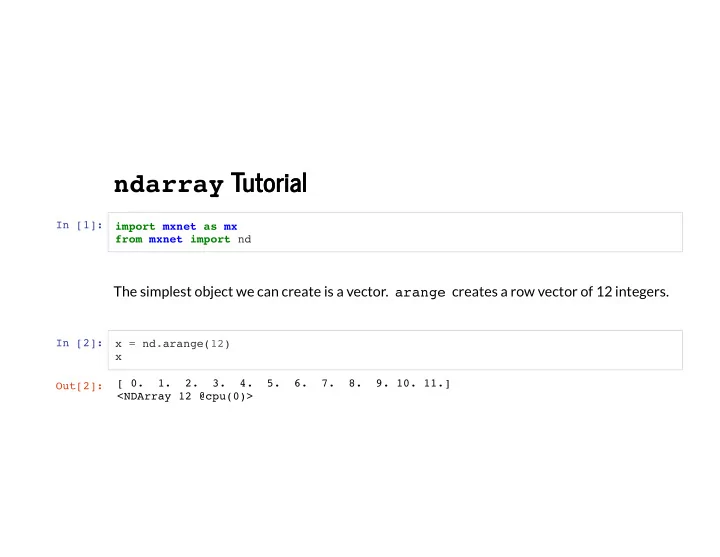
In [1]: import mxnet as mx from mxnet import nd

The simplest object we can create is a vector. arange creates a row vector of 12 integers.

In [2]: x = nd.arange(12) x Out[2]: [ 0. 1. 2. 3. 4. 5. 6. 7. 8. 9. 10. 11.] <NDArray 12 @cpu(0)>

We can get the NDArray instance shape through the shape property.

In [3]: x.shape

We can also get the total number of elements in the NDArray instance through the size property.

In [4]: x.size Out[3]: (12,) Out[4]: 12

The reshape function change the shape of the line vector x to (3, 4), which is a matrix of 3 rows and 4 columns.

In [5]: x = x.reshape((3, 4)) x

We can use -1 to ll in defaults. x.reshape((3, 4)) is equivalent to x.reshape((-1, 4)) and x.reshape((3, -1)) .

Out[5]: [[ 0. 1. 2. 3.] [ 4. 5. 6. 7.] [ 8. 9. 10. 11.]] <NDArray 3x4 @cpu(0)>

The empty method grabs some memory. This is uninitialized.

In [6]: nd.empty((3, 4))

Typically we want all zeros . To create a tensor of shape (2, 3, 4)

In [7]: nd.zeros((2, 3, 4)) Out[6]: [[0. 0. 0. 0.] [0. 0. 0. 0.] [0. 0. 0. 0.]] <NDArray 3x4 @cpu(0)> Out[7]: [[[0. 0. 0. 0.] [0. 0. 0. 0.] [0. 0. 0. 0.]] [[0. 0. 0. 0.] [0. 0. 0. 0.] [0. 0. 0. 0.]]] <NDArray 2x3x4 @cpu(0)>

Creating tensors with each element being 1 works via

In [8]: nd.ones((2, 3, 4))

We can also specify the value of each element in the NDArray that needs to be created through a Python list.

In [9]: y = nd.array([[2, 1, 4, 3], [1, 2, 3, 4], [4, 3, 2, 1]]) y Out[8]: [[[1. 1. 1. 1.] [1. 1. 1. 1.] [1. 1. 1. 1.]] [[1. 1. 1. 1.] [1. 1. 1. 1.] [1. 1. 1. 1.]]] <NDArray 2x3x4 @cpu(0)> Out[9]: [[2. 1. 4. 3.] [1. 2. 3. 4.] [4. 3. 2. 1.]] <NDArray 3x4 @cpu(0)>

In some cases, we need to randomly generate the value of each element in the NDArray. This is especially common when we intend to use the array as a parameter in a neural

• network. The following creates an NDArray with a shape of (3,4). Each of its elements is

randomly sampled in a normal distribution with zero mean and unit variance.

In [10]: nd.random.normal(0, 1, shape=(3, 4)) Out[10]: [[ 1.1630787 0.4838046 0.29956347 0.15302546] [-1.1688148 1.5580711 -0.5459446 -2.3556297 ] [ 0.5414402 2.6785066 1.2546344 -0.54877394]] <NDArray 3x4 @cpu(0)>

Operations Operations

Common standard arithmetic operators (+,-,/,\*,\*\*) have all been lifted to element-wise operations for identically-shaped tensors.

In [11]: x = nd.array([1, 2, 4, 8]) y = nd.ones_like(x) * 2 print('x =', x) print('x + y', x + y) print('x - y', x - y) print('x * y', x * y) print('x / y', x / y) x = [1. 2. 4. 8.] <NDArray 4 @cpu(0)> x + y [ 3. 4. 6. 10.] <NDArray 4 @cpu(0)> x - y [-1. 0. 2. 6.] <NDArray 4 @cpu(0)> x * y [ 2. 4. 8. 16.] <NDArray 4 @cpu(0)> x / y [0.5 1. 2. 4. ] <NDArray 4 @cpu(0)>

Many more operations can be applied element-wise, such as exponentiation:

In [12]: x.exp() Out[12]: [2.7182817e+00 7.3890562e+00 5.4598148e+01 2.9809580e+03] <NDArray 4 @cpu(0)>

In addition to computations by element, we can also use the dot function for matrix

• perations. To perform matrix multiplication we dene x as a matrix of 3 rows and 4

columns, and y is transposed into a matrix of 4 rows and 3 columns.

In [13]: x = nd.arange(12).reshape((3,4)) y = nd.array([[2, 1, 4, 3], [1, 2, 3, 4], [4, 3, 2, 1]]) nd.dot(x, y.T) Out[13]: [[ 18. 20. 10.] [ 58. 60. 50.] [ 98. 100. 90.]] <NDArray 3x3 @cpu(0)>

We can also merge multiple NDArrays. For that, we need to tell the system along which dimension to merge. The example below merges two matrices along dimension 0 (along rows) and dimension 1 (along columns) respectively.

In [14]: nd.concat(x, y, dim=0) nd.concat(x, y, dim=1) Out[14]: [[ 0. 1. 2. 3. 2. 1. 4. 3.] [ 4. 5. 6. 7. 1. 2. 3. 4.] [ 8. 9. 10. 11. 4. 3. 2. 1.]] <NDArray 3x8 @cpu(0)>

Just like in Numpy, we can construct binary NDarrays by a logical statement. Take x == y as an example. If x and y are equal for some entry, the new NDArray has a value of 1 at the same position; otherwise, it is 0.

In [15]: x == y Out[15]: [[0. 1. 0. 1.] [0. 0. 0. 0.] [0. 0. 0. 0.]] <NDArray 3x4 @cpu(0)>

Summing over the NDArray yields an NDArray with one element.

In [16]: x.sum()

We can transform the result into a scalar in Python using the asscalar function. In the following example, the norm of x yields a single element NDArray. The nal result is transformed into a scalar.

In [17]: x.norm().asscalar() Out[16]: [66.] <NDArray 1 @cpu(0)> Out[17]: 22.494442

Broadcast Mechanism Broadcast Mechanism

If shapes of arrays differ a broadcasting mechanism is used (see NumPy): rst, copy the elements appropriately so that both NDArrays have the same shape, then carry out

• perations by element.

In [18]: a = nd.arange(3).reshape((3, 1)) b = nd.arange(2).reshape((1, 2)) a, b Out[18]: ( [[0.] [1.] [2.]] <NDArray 3x1 @cpu(0)>, [[0. 1.]] <NDArray 1x2 @cpu(0)>)

Since a and b are (3x1) and (1x2) matrices respectively, their shapes do not match up if we want to add them. NDArray addresses this by 'broadcasting' the entries of both matrices into a larger (3x2) matrix as follows: for matrix a it replicates the columns, for matrix b it replicates the rows before adding up both element-wise.

In [19]: a + b Out[19]: [[0. 1.] [1. 2.] [2. 3.]] <NDArray 3x2 @cpu(0)>

Indexing and Slicing Indexing and Slicing

Just like in any other Python array, elements in an NDArray can be accessed by its index. In good Python tradition the rst element has index 0 and ranges are specied to include the rst but not the last. By this logic 1:3 selects the second and third element. Let's try this

• ut by selecting the respective rows in a matrix.

In [20]: x[1:3] Out[20]: [[ 4. 5. 6. 7.] [ 8. 9. 10. 11.]] <NDArray 2x4 @cpu(0)>

Beyond reading we can also write elements of a matrix.

In [21]: x[1, 2] = 9 x

If we want to assign multiple elements the same value, we simply index all of them and then assign them the value.

In [22]: x[0:2, :] = 12 x Out[21]: [[ 0. 1. 2. 3.] [ 4. 5. 9. 7.] [ 8. 9. 10. 11.]] <NDArray 3x4 @cpu(0)> Out[22]: [[12. 12. 12. 12.] [12. 12. 12. 12.] [ 8. 9. 10. 11.]] <NDArray 3x4 @cpu(0)>

Saving Memory Saving Memory

We allocated new memory for each operation. For example, if we write y = x + y , we will dereference the matrix that y used to point to and instead point it at the newly allocated memory. After running y = y + x , we'll nd that id(y) points to a different

• location. That's because Python rst evaluates y + x , allocating new memory for the

result and then subsequently redirects y to point at this new location.

In [23]: before = id(y) y = y + x id(y) == before Out[23]: False

In-place operations in MXNet are easy. We can assign the result of an operation to a previously allocated array with slice notation, e.g., y[:] = <expression> .

In [24]: z = y.zeros_like() print('id(z):', id(z)) z[:] = x + y print('id(z):', id(z)) id(z): 4553727616 id(z): 4553727616

While this looks pretty, x+y here will still allocate a temporary buffer to store the result of x+y before copying it to y[:] . To make even better use of memory, we invoke elemwise_add directly.

In [25]: before = id(z) nd.elemwise_add(x, y, out=z) id(z) == before Out[25]: True

If the value of x is not reused in subsequent programs, we can also use x[:] = x + y

• r x += y to reduce the memory overhead of the operation.

In [26]: before = id(x) x += y id(x) == before Out[26]: True

Mutual Transformation of NDArray and NumPy Mutual Transformation of NDArray and NumPy

The converted arrays do not share memory. This minor inconvenience is quite important: when you perform operations on the CPU or one of the GPUs, you don't want MXNet having to wait whether NumPy might want to be doing something else with the same chunk

• f memory.

In [27]: import numpy as np a = x.asnumpy() print(type(a)) b = nd.array(a) print(type(b)) <class 'numpy.ndarray'> <class 'mxnet.ndarray.ndarray.NDArray'>