autograd January 31, 2019 1 Automatic Differentiation 1.1 Import - PDF document

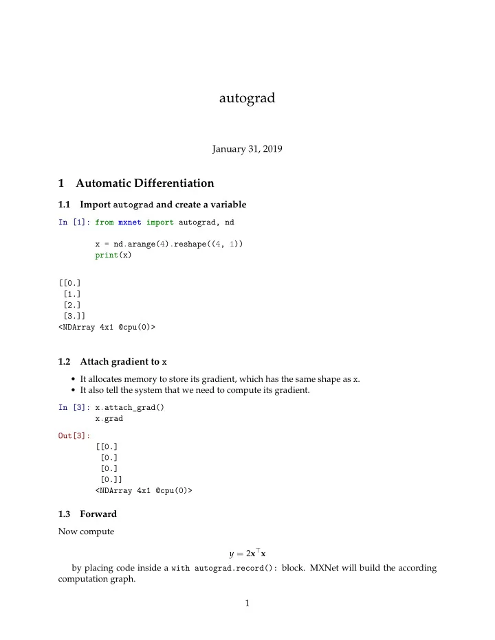
autograd January 31, 2019 1 Automatic Differentiation 1.1 Import autograd and create a variable In [1]: from mxnet import autograd, nd x = nd.arange(4).reshape((4, 1)) print(x) [[0.] [1.] [2.] [3.]] <NDArray 4x1 @cpu(0)> 1.2 Attach gradient to x • It allocates memory to store its gradient, which has the same shape as x . • It also tell the system that we need to compute its gradient. In [3]: x.attach_grad() x.grad Out[3]: [[0.] [0.] [0.] [0.]] <NDArray 4x1 @cpu(0)> 1.3 Forward Now compute y = 2 x ⊤ x by placing code inside a with autograd.record(): block. MXNet will build the according computation graph. 1

In [4]: with autograd.record(): y = 2 * nd.dot(x.T, x) y Out[4]: [[28.]] <NDArray 1x1 @cpu(0)> 1.4 Backward In [5]: y.backward() 1.5 Get the gradient Given y = 2 x ⊤ x , we know ∂ y ∂ x = 4 x Now verify the result: In [6]: print((x.grad - 4 * x).norm().asscalar() == 0) print(x.grad) True [[ 0.] [ 4.] [ 8.] [12.]] <NDArray 4x1 @cpu(0)> 1.6 Backward on non-scalar y.backward() equals to y.sum().backward() In [7]: with autograd.record(): y = 2 * x * x print(y.shape) y.backward() print(x.grad) (4, 1) [[ 0.] [ 4.] [ 8.] [12.]] <NDArray 4x1 @cpu(0)> 2

1.7 Training mode and prediction mode The record scope will alter the mode by assuming that gradient is only required for training. It’s necessary since some layers, e.g. batch normalization, behavior differently in the training and prediction modes. In [7]: print(autograd.is_training()) with autograd.record(): print(autograd.is_training()) False True 1.8 Computing the hradient of Python control flow Autograd also works with Python functions and control flows. In [10]: def f(a): b = a * 2 while b.norm().asscalar() < 1000: b = b * 2 if b.sum().asscalar() > 0: c = b else : c = 100 * b return c 1.9 Function behaviors depends on inputs In [11]: a = nd.random.normal(shape=1) a.attach_grad() with autograd.record(): d = f(a) d.backward() 1.10 Verify the results f is piecewise linear in its input a . There exists g such as f ( a ) = ga and ∂ f ∂ a = g . Verify the result: In [12]: print(a.grad == (d / a)) [1.] <NDArray 1 @cpu(0)> 3

1.11 Head gradients and the chain rule ∂ y ∂ x . y.backward() will only compute ∂ y We can break the chain rule manually. Assume ∂ z ∂ x = ∂ z ∂ x . ∂ y To get ∂ z ∂ x , we can first compute ∂ z ∂ y , and then pass it as head gradient to y.backward . In [11]: with autograd.record(): y = x * 2 y.attach_grad() with autograd.record(): z = y * x z.backward() # y.grad = \partial z / \partial y y.backward(y.grad) x.grad == 2*x # x.grad = \partial z / \partial x Out[11]: [[1.] [1.] [1.] [1.]] <NDArray 4x1 @cpu(0)> 4