
SLIDE 1
Concise Implementation of Linear Regression Concise Implementation of Linear Regression
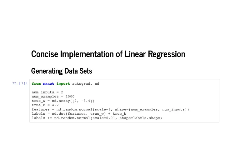
Generating Data Sets Generating Data Sets
In [1]: from mxnet import autograd, nd num_inputs = 2 num_examples = 1000 true_w = nd.array([2, -3.4]) true_b = 4.2 features = nd.random.normal(scale=1, shape=(num_examples, num_inputs)) labels = nd.dot(features, true_w) + true_b labels += nd.random.normal(scale=0.01, shape=labels.shape)