Multiple change-point analysis k k k f s g f h g - - PDF document

SLIDE 1

Multiple change-point analysis

A Bayesian approach to change-point analysis for point processes

y

• y
• y

n : combines Poisson-process likelihood: py jx

• exp

f P n i log xy i

• R

L

• xtdtg

prior model for step function xt,

• t
• L,

representing intensity Prior model: represent step function by

k

• fs

j g k j

• fh

j g k j

• :

xt

• P

j h j I s j s j

• t:

number of steps k: Poisson(), step heights h j: Gamma(

• ),

step positions s j: psjk

• Q

j s j

• s

j ,

all independent.

18

MCMC for step functions

• k
• fs

j g k j

• fh

j g k j

• I will use four moves:

(a) Metropolis change to a randomly chosen step height

h j.

(b) Metropolis change to a randomly chosen step position

s j.

(c) Jump move: birth/death of steps – birth: choose new step position

s at

random, split current step height

h into two: h

• h
• – death: choose step at random to kill,

combine current step heights

h

• h
• into
• ne:

h

(d) Update hyperparameters

,

• 19

Birth and death of steps

j-

h hj+ s* sj sj-1 h

h w

• h

w

• h

w

• w
• h

w

• s
• u
• h
• h
• w
• w
• 20

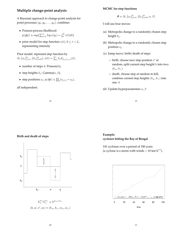
Example: cyclones hitting the Bay of Bengal 141 cyclones over a period of 100 years (a cyclone is a storm with winds

• km h

).

time 20 40 60 80 100

.. . .. . . . .. ... . .. . .. . . . . .. . ... . . ... . . . .. . .. . . .. .. . . ... . . . . . .... . ... .. . . . . . .. .. . .. . .. .. .... . . . . .. . . .. . .. . . . . . . . . . . . . . . . .. . . . . . .. . . .. . . . .. . . . . . .

21

SLIDE 2

Choices of hyperparameters:

Prior on k: Poisson(), with

• .

Prior on h j: Gamma(,), with

–

• –
• nL

Sample of step functions from the posterior:

time intensity 20 40 60 80 100 1 2 3 22

Posterior for the number of change points

k

• k

probability 2 4 6 8 10 12 0.0 0.10 0.20

Zero change points is ruled out;

k

• r

more

probable than under the prior.

23

Posterior density estimates for change-point positions

time density 20 40 60 80 100 0.0 0.05 0.10 0.15 24

Model-averaged estimate:

E xjy

• time

intensity 20 40 60 80 100 0.0 0.5 1.0 1.5 2.0 2.5

.. . .. . . . .. ... . .. . .. . . . . .. . ... . . ... . . . .. . .. . . .. .. . . ... . . . . . .... . ... .. . . . . . .. .. . .. . .. .. .... . . . . .. . . .. . .. . . . . . . . . . . . . . . . .. . . . . . .. . . .. . . . .. . . . . . . (the expectation of a random step function is not a step function).

25

SLIDE 3

Ordinary smoothing methods (in this case a kernel smoother) can’t match that mean curve

time intensity 20 40 60 80 100 0.0 0.5 1.0 1.5 2.0 2.5

.. . .. . . . .. ... . .. . .. . . . . .. . ... . . ... . . . .. . .. . . ... . . ... . . . . . .... . ... .. . . . . . .. .. . .. . .. .. .... . . . . .. . . .. . .. . . . . . . . . . . . . . . . .. . . . . . .. . . .. . . . .. . . . . . . – fixed-bandwidth smoothers either over-smooth the steps, or under-smooth the plateaux.

26