moment generating functions
play

moment generating functions powerful math tricks for dealing with - PowerPoint PPT Presentation

moment generating functions powerful math tricks for dealing with distributions we wont do much with it, but mentioned/used in book, so a very brief introduction: the k th moment of r.v. X is E[X k ]; M.G.F. is M(t) = E[e tX ] 1 the law


  1. moment generating functions 
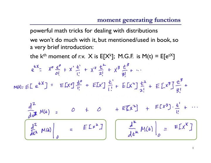
powerful math tricks for dealing with distributions we won’t do much with it, but mentioned/used in book, so a very brief introduction: the k th moment of r.v. X is E[X k ]; M.G.F. is M(t) = E[e tX ] 1

  2. the law of large numbers & the CLT 2

  3. weak law of large numbers i.i.d. (independent, identically distributed) random vars X 1 , X 2 , X 3 , … X i has μ = E[X i ] < ∞ and σ 2 = Var[X i ] Consider the empirical mean : The Weak Law of Large Numbers: For any ε > 0, as n → ∞ 3

  4. weak law of large numbers For any ε > 0, as n → ∞ Proof: ( assume σ 2 < ∞ ) By Chebyshev inequality, 4

  5. strong law of large numbers i.i.d. (independent, identically distributed) random vars X 1 , X 2 , X 3 , … X i has μ = E[X i ] < ∞ Strong Law ⇒ Weak Law (but not vice versa) Strong law implies that for any ε > 0, there are only finite number of n such that the weak law condition is violated. 5

  6. diffusion http://en.wikipedia.org/wiki/Law_of_large_numbers 6

  7. the law of large numbers Note: D n = E[ | Σ 1 ≤ i ≤ n (X i - μ ) | ] grows with n, but D n /n → 0 Justifies the “frequency” interpretation of probability “Regression toward the mean” Gambler’s fallacy: “I’m due for a win!” “Result will usually be close to the mean” Many web demos, e.g. http://stat-www.berkeley.edu/~stark/Java/Html/lln.htm 7

  8. normal random variable • X is a normal random variable X ~ N( μ , σ 2 ) 8

  9. normal random variable X is a normal random variable X ~ N( μ , σ 2 ) Z ~ N(0,1) “standard (or unit) normal” Use Φ (z) to denote CDF, i.e. no closed form ☹ 9

  10. the central limit theorem (CLT) i.i.d. (independent, identically distributed) random vars X 1 , X 2 , X 3 , … X i has μ = E[X i ] and σ 2 = Var[X i ] As n → 1, Restated: As n → ∞ , 10

  11. CLT in the real world CLT is the reason many things appear normally distributed Many quantities = sums of (roughly) independent random vars Exam scores: sums of individual problems People’s heights: sum of many genetic & environmental factors Measurements: sums of various small instrument errors ... 11

  12. in the real world… Human height is approximately normal. Frequency Why might that be true? R.A. Fisher (1918) noted it would follow from CLT if height Male Height in Inches were the sum of many independent random effects, e.g. many genetic factors (plus some environmental ones like diet) . I.e., suggested part of mechanism by looking at shape of the curve. 12

  13. CLT convergence 13

  14. Chernoff bound was CLT (for binomial) in disguise • Suppose X ~ Bin(n,p) • μ = E[X] = pn • Chernoff bound: 14

  15. rolling more dice • Roll 10 6-sided dice • X = total value of all 10 dice • Win if: X ≤ 25 or X ≥ 45 • Roll… 15

Download Presentation
Download Policy: The content available on the website is offered to you 'AS IS' for your personal information and use only. It cannot be commercialized, licensed, or distributed on other websites without prior consent from the author. To download a presentation, simply click this link. If you encounter any difficulties during the download process, it's possible that the publisher has removed the file from their server.

Recommend


More recommend