Minimum Spanning Tree Minimum spanning tree. Given a connected - - PowerPoint PPT Presentation

3

Minimum Spanning Tree

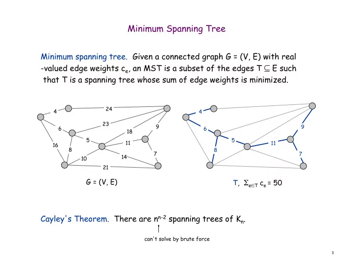
Minimum spanning tree. Given a connected graph G = (V, E) with real

• valued edge weights ce, an MST is a subset of the edges T ⊆ E such

that T is a spanning tree whose sum of edge weights is minimized. Cayley's Theorem. There are nn-2 spanning trees of Kn.

5 23 10 21 14 24 16 6 4 18 9 7 11 8 5 6 4 9 7 11 8

G = (V, E) T, Σe∈T ce = 50

can't solve by brute force

4

Applications

MST is fundamental problem with diverse applications.



Network design.

– telephone, electrical, hydraulic, TV cable, computer, road



Approximation algorithms for NP-hard problems.

– traveling salesperson problem, Steiner tree



Indirect applications.

– max bottleneck paths – LDPC codes for error correction – image registration with Renyi entropy – learning salient features for real-time face verification – reducing data storage in sequencing amino acids in a protein – model locality of particle interactions in turbulent fluid flows – autoconfig protocol for Ethernet bridging to avoid cycles in a network



Cluster analysis.

5

Greedy Algorithms

Kruskal's algorithm. Start with T = φ. Consider edges in ascending

• rder of cost. Insert edge e in T unless doing so would create a cycle.

Reverse-Delete algorithm. Start with T = E. Consider edges in descending order of cost. Delete edge e from T unless doing so would disconnect T. Prim's algorithm. Start with some root node s and greedily grow a tree T from s outward. At each step, add the cheapest edge e to T that has exactly one endpoint in T.

• Remark. All three algorithms produce an MST.

6

Greedy Algorithms

Simplifying assumption. All edge costs ce are distinct. Cut property. Let S be any subset of nodes, and let e be the min cost edge with exactly one endpoint in S. Then the MST contains e. Cycle property. Let C be any cycle, and let f be the max cost edge belonging to C. Then the MST does not contain f.

f

C S e is in the MST

e

f is not in the MST

7

Cycles and Cuts

• Cycle. Set of edges the form a-b, b-c, c-d, …, y-z, z-a.
• Cutset. A cut is a subset of nodes S. The corresponding cutset D is

the subset of edges with exactly one endpoint in S.

Cycle C = 1-2, 2-3, 3-4, 4-5, 5-6, 6-1 1 3 8 2 6 7 4 5 Cut S = { 4, 5, 8 } Cutset D = 5-6, 5-7, 3-4, 3-5, 7-8 1 3 8 2 6 7 4 5

8

Cycle-Cut Intersection

• Claim. A cycle and a cutset intersect in an even number of edges.
• Pf. (by picture)

1 3 8 2 6 7 4 5

S V - S C

Cycle C = 1-2, 2-3, 3-4, 4-5, 5-6, 6-1 Cutset D = 3-4, 3-5, 5-6, 5-7, 7-8 Intersection = 3-4, 5-6

9

Greedy Algorithms

Simplifying assumption. All edge costs ce are distinct. Cut property. Let S be any subset of nodes, and let e be the min cost edge with exactly one endpoint in S. Then the MST T* contains e.

• Pf. (exchange argument)

 Suppose e does not belong to T*, and let's see what happens.  Adding e to T* creates a cycle C in T*.  Edge e is both in the cycle C and in the cutset D corresponding to S

⇒ there exists another edge, say f, that is in both C and D.

 T' = T* ∪ { e } - { f } is also a spanning tree.  Since ce < cf, cost(T') < cost(T*).  This is a contradiction. ▪

f T* e

S

10

Greedy Algorithms

Simplifying assumption. All edge costs ce are distinct. Cycle property. Let C be any cycle in G, and let f be the max cost edge belonging to C. Then the MST T* does not contain f.

• Pf. (exchange argument)

 Suppose f belongs to T*, and let's see what happens.  Deleting f from T* creates a cut S in T*.  Edge f is both in the cycle C and in the cutset D corresponding to S

⇒ there exists another edge, say e, that is in both C and D.

 T' = T* ∪ { e } - { f } is also a spanning tree.  Since ce < cf, cost(T') < cost(T*).  This is a contradiction. ▪

f T* e

S

11

Prim's Algorithm: Proof of Correctness

Prim's algorithm. [Jarník 1930, Dijkstra 1957, Prim 1959]

 Initialize S = any node.  Apply cut property to S.  Add min cost edge in cutset corresponding to S to T, and add one

new explored node u to S.

S

12

Implementation: Prim's Algorithm

Prim(G, c) { foreach (v ∈ V) a[v] ← ∞ Initialize an empty priority queue Q foreach (v ∈ V) insert v onto Q Initialize set of explored nodes S ← φ while (Q is not empty) { u ← delete min element from Q S ← S ∪ { u } foreach (edge e = (u, v) incident to u) if ((v ∉ S) and (ce < a[v])) decrease priority a[v] to ce }

• Implementation. Use a priority queue ala Dijkstra.

 Maintain set of explored nodes S.  For each unexplored node v, maintain attachment cost a[v] = cost of

cheapest edge v to a node in S.

 O(n2) with an array; O(m log n) with a binary heap.

13

Kruskal's Algorithm: Proof of Correctness

Kruskal's algorithm. [Kruskal, 1956]



Consider edges in ascending order of weight.



Case 1: If adding e to T creates a cycle, discard e according to cycle property.



Case 2: Otherwise, insert e = (u, v) into T according to cut property where S = set of nodes in u's connected component.

Case 1

v u

Case 2

e e

S

14

Implementation: Kruskal's Algorithm

Kruskal(G, c) { Sort edges weights so that c1 ≤ c2 ≤ ... ≤ cm. T ← φ foreach (u ∈ V) make a set containing singleton u for i = 1 to m (u,v) = ei if (u and v are in different sets) { T ← T ∪ {ei} merge the sets containing u and v } return T }

• Implementation. Use the union-find data structure.

 Build set T of edges in the MST.  Maintain set for each connected component.  O(m log n) for sorting and O(m α (m, n)) for union-find.

are u and v in different connected components? merge two components m ≤ n2 ⇒ log m is O(log n) essentially a constant

15

Lexicographic Tiebreaking

To remove the assumption that all edge costs are distinct: perturb all edge costs by tiny amounts to break any ties.

• Impact. Kruskal and Prim only interact with costs via pairwise
• comparisons. If perturbations are sufficiently small, MST with

perturbed costs is MST with original costs.

• Implementation. Can handle arbitrarily small perturbations implicitly

by breaking ties lexicographically, according to index.

boolean less(i, j) { if (cost(ei) < cost(ej)) return true else if (cost(ei) > cost(ej)) return false else if (i < j) return true else return false }

e.g., if all edge costs are integers, perturbing cost of edge ei by i / n2

4.7 Clustering

Outbreak of cholera deaths in London in 1850s. Reference: Nina Mishra, HP Labs

17

Clustering

• Clustering. Given a set U of n objects labeled p1, …, pn, classify into

coherent groups. Distance function. Numeric value specifying "closeness" of two objects. Fundamental problem. Divide into clusters so that points in different clusters are far apart.

 Routing in mobile ad hoc networks.  Identify patterns in gene expression.  Document categorization for web search.  Similarity searching in medical image databases  Skycat: cluster 109 sky objects into stars, quasars, galaxies.

photos, documents. micro-organisms number of corresponding pixels whose intensities differ by some threshold

18

Clustering of Maximum Spacing

k-clustering. Divide objects into k non-empty groups. Distance function. Assume it satisfies several natural properties.

 d(pi, pj) = 0 iff pi = pj (identity of indiscernibles)  d(pi, pj) ≥ 0

(nonnegativity)

 d(pi, pj) = d(pj, pi)

(symmetry)

• Spacing. Min distance between any pair of points in different clusters.

Clustering of maximum spacing. Given an integer k, find a k-clustering

• f maximum spacing.

spacing

k = 4

19

Greedy Clustering Algorithm

Single-link k-clustering algorithm.

 Form a graph on the vertex set U, corresponding to n clusters.  Find the closest pair of objects such that each object is in a

different cluster, and add an edge between them.

 Repeat n-k times until there are exactly k clusters.

Key observation. This procedure is precisely Kruskal's algorithm (except we stop when there are k connected components).

• Remark. Equivalent to finding an MST and deleting the k-1 most

expensive edges.

20

Greedy Clustering Algorithm: Analysis

• Theorem. Let C* denote the clustering C*1, …, C*k formed by deleting the

k-1 most expensive edges of a MST. C* is a k-clustering of max spacing.

• Pf. Let C denote some other clustering C1, …, Ck.

 The spacing of C* is the length d* of the (k-1)st most expensive edge.  Let pi, pj be in the same cluster in C*, say C*r, but different clusters

in C, say Cs and Ct.

 Some edge (p, q) on pi-pj path in C*r spans two different clusters in C.  All edges on pi-pj path have length ≤ d*

since Kruskal chose them.

 Spacing of C is ≤ d* since p and q

are in different clusters. ▪

p q

pi

pj

Cs Ct C*r