SLIDE 1
MAV Annual Conference 2018 Further Maths exams: using the CAS calculator efficiently and effectively
Presenter: Kevin McMenamin | e: kxm@mentonegrammar.net
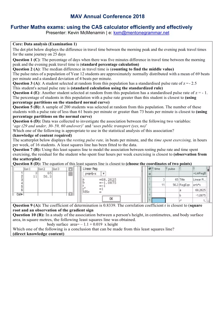
Core: Data analysis (Examination 1) The dot plot below displays the difference in travel time between the morning peak and the evening peak travel times for the same journey on 25 days Question 1 (C): The percentage of days when there was five minutes difference in travel time between the morning peak and the evening peak travel time is (standard percentage calculation) Question 2 (A): The median difference in travel time is (counting to find the middle value) The pulse rates of a population of Year 12 students are approximately normally distributed with a mean of 69 beats per minute and a standard deviation of 4 beats per minute. Question 3 (A): A student selected at random from this population has a standardised pulse rate of z = - 2.5 This student's actual pulse rate is (standard calculation using the standardized rule) Question 4 (E): Another student selected at random from this population has a standardised pulse rate of z = - 1. The percentage of students in this population with a pulse rate greater than this student is closest to (using percentage partitions on the standard normal curve) Question 5 (B): A sample of 200 students was selected at random from this population. The number of these students with a pulse rate of less than 61 beats per minute or greater than 73 beats per minute is closest to (using percentage partitions on the normal curve) Question 6 (D): Data was collected to investigate the association between the following two variables: ‘age (29 and under, 30- 59, 60 and over)’ and ‘uses public transport (yes, no)’ Which one of the following is appropriate to use in the statistical analysis of this association? (knowledge of content required) The scatterplot below displays the resting pulse rate, in beats per minute, and the time spent exercising, in hours per week, of 16 students. A least squares line has been fitted to the data. Question 7 (B): Using this least squares line to model the association between resting pulse rate and time spent exercising, the residual for the student who spent four hours per week exercising is closest to (observation from the scatterplot) Question 8 (D): The equation of this least squares line is closest to (choose the coordinates of two points) Question 9 (A): The coefficient of determination is 0.8339. The correlation coefficient r is closest to (square root and an observation of the gradient sign Question 10 (B): In a study of the association between a person's height, in centimetres, and body surface area, in square metres, the following least squares line was obtained. body surface area= – 1.1 + 0.019 x height Which one of the following is a conclusion that can be made from this least squares line? (direct knowledge content)
SLIDE 2 Question 11 (A) : Freya uses the following data to generate the scatterplot below. The scatterplot shows that the data is non-linear. To linearise the data, Freya applies a reciprocal transformation to the variable y. She then fits a least squares line to the transformed data. With x as the explanatory variable, the equation of this least squares line is closest to Question 12 (E): A log 10 (y) transformation was used to linearise a set of non-linear bivariate data. A least squares line was then fitted to the transformed data. The equation of this least squares line is log10 ( y) = 3.1 - 2.3x This equation is used to predict the value of y when x = 1.1 The value of y is closest to Question 13 (D): The statistical analysis of a set of bivariate data involving variables x and y resulted in the information displayed in the table below (simple calculation of
y x
s b r s =
) Question 14 (C): A least squares line is fitted to a set of bivariate data. Another least squares line is fitted with response and explanatory variables reversed. Which one of the following statistics will not change in value? (knowledge based question) Question 15 (B): The table below shows the monthly profit, in dollars, of a new coffee shop for the first nine months
Month Jan. Feb. Mar. Apr. May June July Aug. Sept. Profit($) 2890 1978 2402 2456 4651 3456 2823 2678 2345 Using four-mean smoothing with centring, the smoothed profit for May is closest to (multiple additions) Question 16 (C): The quarterly sales figures for a large suburban garden centre, in millions of dollars, for 2016 and 2017 are displayed in the table below. Year Quarter 1 Quarter 2 Quarter 3 Quarter 4 2016 1.73 2.87 3.34 1.23 2017 1.03 2.45 2.05 0.78 Using these sales figures, the seasonal index for Quarter 3 is closest to
SLIDE 3 Core: Data analysis (Examination 2) Question 1 Traffic congestion can lead to an increase in travel times in cities. The dot plot and boxplot below both show the increase in travel time due to traffic congestion, in minutes per day, for the 23 UK cities.
- g. The data value 52 is below the upper fence and is not an outlier. Determine the value of the upper fence.
Upper = 39 + 1.5 × (39 – 30) = 52.5 Question 2c A least squares line is to be fitted to the data with the aim of predicting evening congestion level from morning congestion level. The equation of this line is evening congestion level = 8.48 + 0.922 × morning congestion level Use the equation of the least squares line to predict the evening congestion level when the morning congestion level is 60%. Simple calculation: 8.49 + 0.922 × 60 = 63.8 Question 2d Determine the residual value when the equation of the least squares line is used to predict the evening congestion level when the morning congestion level is 47%. Round your answer to one decimal place. Question 3b. A least squares line is used to model the trend in the time series plot for Sydney. The equation is congestion level = –2280 + 1.15 × year
- i. Draw this least squares line on the time series plot on page 8.
Note: choose 2 points far apart and evaluate the predicted value Plot the two points (2008 , 29,2) and (2016 , 38.4) Question 3b
- ii. Use the equation of the least squares line to determine the average rate of increase in percentage congestion level
for the period 2008 to 2016 in Sydney.
- iii. Use the least squares line to predict when the percentage congestion level in Sydney will be 43%.
SLIDE 4 Question 3d Year 2008 2009 2010 2011 2012 2013 2014 2015 2016 Melbourne 25 26 26 27 28 28 29 29 33 Use the data in Table 4 to determine the equation of the least squares line that can be used to model the trend in the data for Melbourne. The variable year is the explanatory variable. Write the values of the intercept and the slope of this least squares line. Round both values to four significant figures. Recursion and Financial Modelling (Exam 1) The value of an annuity investment, in dollars, after n years,
1 n
V + can be modelled by the recurrence relation shown
below.
1
46000 , 1.0034 500
n n
V V V
+
= = +
Question 18 (C) Between the second and third years, the increase in the value of this investment is closest to Question 19 (D) Daniel borrows $5000, which he intends to repay fully in a lump sum after one year. The annual interest rate and compounding period for five different compound interest loans are given below: Loan I - 12.6% per annum, compounding weekly Loan II - 12.8% per annum, compounding weekly Loan III - 12.9% per annum, compounding weekly Loan IV - 12.7% per annum, compounding quarterly Loan V - 13.2% per annum, compounding quarterly When fully repaid, the loan that will cost Daniel the least amount of money is
SLIDE 5 1
Question 21 (B) Which one of the following recurrence relations could be used to model the value of a perpetuity investment,
1 n
P + ,
after n months? Question 22 (E) Adam has a home loan with a present value of $175 260.56 The interest rate for Adam's loan is 3.72% per annum, compounding monthly. His monthly repayment is $3200. The loan is to be fully repaid after five years. Adam knows that the loan cannot be exactly repaid with 60 repayments of $3200. To solve this problem, Adam will make 59 repayments of $3200. He will then adjust the value of the final repayment so that the loan is fully repaid with the 60th repayment. The value of the 60th repayment will be closest to Final payment: 3200 + 368.12 =$3568.12 Question 23 (A)
Five lines of an amortisation table for a reducing balance loan with monthly repayments are shown below. The interest rate for this loan changed immediately before repayment number 28. This change in interest rate is best described as
SLIDE 6 Question 24 (E) Mariska plans to retire from work 10 years from now. Her retirement goal is to have a balance of $600 000 in an annuity investment at that time. The present value of this annuity investment is $265 298.48, on which she earns interest at the rate of 3.24% per annum, compounding monthly. To make this investment grow faster, Mariska will add a $1000 payment at the end of every month. Two years from now, she expects the interest rate of this investment to fall to 3.20% per annum, compounding
- monthly. It is expected to remain at this rate until Mariska retires.
When the interest rate drops, she must increase her monthly payment if she is to reach her retirement goal. The value of this new monthly payment will be closest to Recursion and Financial Modelling (Exam 2) Question 4 Julie deposits some money into a savings account that will pay compound interest every month. The balance of Julie’s account, in dollars, after n months,
n
V , can be modelled by the recurrence relation shown below.
1
12000 , 1.0062
n n
V V V
+
= =
- ii. After how many months will the balance of Julie’s account first exceed $12 300?
Question 5 After three years, Julie withdraws $14 000 from her account to purchase a car for her business. For tax purposes, she plans to depreciate the value of her car using the reducing balance method. The value of Julie’s car, in dollars, after n years,
n
C , can be modelled by the recurrence relation shown below.
1
14000 ,
n n
C C R C
+
= = ×
For each of the first three years of reducing balance depreciation, the value of R is 0.85
- b. For the next five years of reducing balance depreciation, the annual rate of depreciation in the value of the car is
changed to 8.6%. What is the value of the car eight years after it was purchased?
SLIDE 7 Question 6 Julie has retired from work and has received a superannuation payment of $492 800. She has two options for investing her money. Option 1 Julie could invest the $492 800 in a perpetuity. She would then receive $887.04 each fortnight for the rest of her life.
- a. At what annual percentage rate is interest earned by this perpetuity?
Option 2 Julie could invest the $492 800 in an annuity, instead of a perpetuity. The annuity earns interest at the rate of 4.32% per annum, compounding monthly. The balance of Julie’s annuity at the end of the first year of investment would be $480 242.25
- b. i. What monthly payment, in dollars, would Julie receive?
- b. ii. How much interest would Julie’s annuity earn in the second year of investment?
Matrices: (Examination 1) Question 1 (D): Which one of the following matrices has a determinant of zero? Question 2: The matrix product of [
]
4 4 2 12 8 ×
Question 5 (B): Liam cycles, runs, swims and walks for exercise several times a month. Each time he cycles, Liam covers a distance of c kilometres. Each time he runs, Liam covers a distance of r kilometres. Each time he swims, Liam covers a distance of s kilometres. Each time he walks, Liam covers a distance of w kilometres. The number of times that Liam cycled, ran, swam and walked each month over a four-month period, and the total distance that Liam travelled in each of those months, are shown in the table below. Number of times in a month Cycle Run Swim Walk Total distance for a month (km) Month 1
5
7 6 8
160
Month 2 8 6 9 7
172
Month 3 7 8 7 6
165
Month 4 8 8
5 5 162
SLIDE 8 Question 7 (E): A study of the antelope population in a wildlife park has shown that antelope regularly move between three locations, east (E), north (N) and west (W). Let
n
A be the state matrix that shows the population of antelope in each location n months after the study began.
The expected population of antelope in each location can be determined by the matrix recurrence rule
1 n n
A TA D
+ =
−
The number of antelope in the west (W) location two months after the study began, as found in the state matrix
2
A , is
closest to Matrices: (Examination 2)
- c. Consider the matrix equation where a = cost of one pie, b = cost of one roll and c = cost of one sandwich.
- i. What is the cost of one sandwich?
Question 8 A public library organised 500 of its members into five categories according to the number of books each member borrows each month. These categories are: J = no books borrowed per month K = one book borrowed per month L = two books borrowed per month M = three books borrowed per month N = four or more books borrowed per month The transition matrix, T, below shows how the number of books borrowed per month by the members is expected to change from month to month. In the long term, which category is expected to have approximately 96 members each month? Question 2 The Westhorn Council must prepare roads for expected population changes in each of three locations: main town (M), villages (V) and rural areas (R). The population of each of these locations in 2018 is shown in matrix
2018
P
below. The expected annual change in population in each location is shown in the table below. Location Main town Villages Rural areas Annual Change Increase by 4% Decrease by 1% Decrease by 2% Write down matrix
2019
P
, which shows the expected population in each location in 2019.
SLIDE 9 The state matrix describing the highway maintenance schedule for the nth year after 2018 is given by
1 n n
S TS
+ =
- c. Complete the state matrix,
1
S , below for the highway maintenance schedule for 2019 (one year after 2018).
In the long term, what percentage of highway each year is expected to have no maintenance (N)? Geometry and Measurement: (Examination 1) Question 1 (B): right angled triangle, finding the hypotenuse:
2 2
8 15 +
Question 2 (A): Area of non-right angles triangle (angle and sides involved):
( )( ) ( )
1 18 26 sin 30 2 A =
Question 3 (C): arc length of a great circle (theory) Question 4 (E): Bearings (theory) Question 5 (C): time zones:
( )
15 30 25 60 × −
Question 6 (C): cosine rule/perimeter of a non-right angled triangle:
( )( ) ( )
2 2 2
5.4 2.8 2 5.4 2.8 cos 75 a = + −
Question 7 (B): area between two sectors:
( )
2 2
1 110 30 9 2 360 × −
Question 8 D): surface area of a cone/Pythagoras:
( )
2
1 ( 2.5 36, ) 3 solve h h π =
/
2 2 2
2.5 x h = +
Geometry and Measurement: (Examination 2) Question 1b: surface area of a cylinder:
( ) ( )( )
2
2 3.4 2 3.4 20.4 π π +
(image given) Question 1ci: volume of a sphere (tennis ball):
( )
3
4 3.4 3 V π =
(image given) Question 1cii: volume of a cylinder:
( ) ( )
2
3.4 20.4 V π =
Question 2a: time zone Question 2bi: small circle radius:
( )
cos 11 6400 r =
(image not given) Question 2bii: small circle/parallel of latitude distance : (
)
123 107 2 6282.41 360 π − × ×
Question 3a. Pythagoras:
( )
2 2 2
4.1 6.4 6.4 5.5 AB = + + +
(image given) Question 3b. Vertical Pythagoras:
( )
2 2 2
2.5 18.8 dist = +
(image not given) Question 3ci: sine rule (ambiguous case):
( ) ( )
sin sin 23.5 | 0 180 20.7 10.4 A A = ≤ ≤
Question 3cii: cosine rule:
( )( ) ( )
2 2 2
20.7 10.4 2 10.4 cos x x A = + −
SLIDE 10
Graphs and Relations: (Examination 1) Question 1 (C): The graph below shows a line intersecting the x-axis at (4, 0) and the y-axis at (0, 2). The gradient of the line is: Question 3 (D) The three inequalities below were used to construct the feasible region for a linear programming problem. x < 3 y < 6 x+ y > 6 A point that lies within this feasible region is Question 4 (B) A team of four students competes in a 4 x 100 m relay race. Each student in the race runs 100 m. The order in which each student runs in the race is shown in the table below. Order Name first Joanne second Elle third Sam fourth Kristen The following line-segment graph represents the race for Joanne, Sam and Kristen, where d is the distance, in metres, from the starting point and t is the recorded time, in seconds. Elle's line segment is missing. The equation representing Elle's line segment is Equation between two points (20,100) and (45,200) Question 6 (E) Amy makes and sells quilts. The fixed cost to produce the quilts is $800. Each quilt costs an additional $35 to make. Amy made and sold a batch of 80 quilts for a profit of $1200. The selling price of each quilt was; Familiarity with: profit – revenue - cost
SLIDE 11
Question 8 (D) A ride-share company has a fee that includes a fixed cost and a cost that depends on both the time spent travelling, in minutes, and the distance travelled, in kilometres. The fixed cost of a ride is $2.55 Judy's ride cost $16.75 and took eight minutes. The distance travelled was 10 km. Pat's ride cost $30.35 and took 20 minutes. The distance travelled was 18 km. Roy's ride took 10 minutes. The distance travelled was 15 km. The cost of Roy's ride was