Math 140 Introductory Statistics The science of learning from data - - PowerPoint PPT Presentation

1

Math 140 Introductory Statistics

Professor Silvia Fernández Chapter 1 Based on the book Statistics in Action by A. Watkins, R. Scheaffer, and G. Cobb.

Statistics

The science of learning from data in the presence of variability.

Our first problem The data in Martin v. Westvaco.

[Source: Martin v. Envelope Division of Westvaco Corp., CA No. 92-03121-MAP, 850 Fed. Supp. 83 (1994).]

2

Statistical Work

Data Exploration

Examination of

data for patterns.

Tools: summary

tables, graphs, averages, etc. Inference (making

inferences from data)

Definition: Deciding

whether or not an

• bserved feature of the

data could reasonably be attributed to chance.

Data from Tables

… …

56 H Engineering Tech II 4 38 H Engineering Tech I 3 25 H Engineering Clerk 2 Age Round … Pay Job Title Row

Cases [rows] Subjects/objects

• f statistical examination

In the example:

• Cases = individual Westvaco employees
• Variables = year of birth, job title, pay, etc.

Variables [columns] Characteristics of each case. It allows us to see the variability

Understanding Variability

To understand how the characteristics of the

cases varies we look at their distribution.

Distribution: What the values are and how

• ften they occur (record of variability)

How can we study the distribution?

By observing the values in each column of the

table.

By graphing the values in a dot plot.

Dot Plots

Each case is represented by a dot located

according to the numerical value of the variable we are investigating.

33 Engineering Tech II 13 35 Engineering Tech II 14 55 Engineering Tech II 12 55 Technical Secretary 11 64 Engineering Tech II 10 55 Engineering Tech II 9 22 Parts Crib Attendant 8 59 Engineering Tech II 7 55 Engineering Tech II 6 53 Engineering Tech II 5 48 Secretary 4 56 Engineering Tech II 3 38 Engineering Tech II 2 25 Engineering Clerk 1 Age Job Title Row

3

Comparing dot plots

Discussion: Exploring the Martin v. Westvaco Data

• D1. Suppose you were on a jury in the Martin
• v. Westvaco case. How would you use the

information in Display 1.1 (The table) to decide if Westvaco tended to lay off older workers (for whatever reason)?

• D2. Compare the plots for the hourly and

salaried workers. Which provides stronger evidence in support of Martin’s claim of age discrimination?

Hourly Salaried

Discussion: Exploring the Martin v. Westvaco Data

• D3. Whenever you think you have a message from data, you

should be careful not to jump to conclusions. The patterns in the Westvaco data might be “real”—they reflect age discrimination

• n the part of management. On the other hand, the patterns

might be the result of chance—management wasn’t discriminating on the basis of age but simply by chance happened to lay off a larger percentage of older workers. What’s your opinion about the Westvaco data: Do the patterns seem “real”—too strong to be explained by chance?

• D4. The analysis up to this point ignores important facts such as

worker qualifications. Suppose Martin makes a convincing case that older workers were more likely to be laid off . It is then up to Westvaco to justify its actions. List several specific reasons Westvaco might give to justify laying off a disproportionate number of older workers.

4

Round by Round

Which display provides stronger support for Martin’s claim that Westvaco discriminated against older workers?

Using Tables to Compare

The summary table shown here classifies salaried

workers using two yes/no questions: Under 40? and Laid off ? (In employment law, 40 is a special age because only those 40 or older belong to what is called the “protected class,” the group covered by the law against age discrimination.)

50 36 18 18 Total 51.9 27 13 14 No 44.4 9 5 4 Yes % Yes Total No Yes Under 40? Laid Off?

Using Tables to Compare

50 36 18 18 Total 51.9 27 13 14 No 44.4 9 5 4 Yes % Yes Total No Yes

• a. Does the pattern in this table support Martin’s claim of age

discrimination? Why or why not?

• b. Construct a similar table for salaried workers, but this time

use 50 instead of 40 to divide the ages. (Your two age groups will be those under 50 and those 50 or older.) Does the evidence in this new table provide stronger or weaker support for Martin’s case? Explain.

Under 40? Laid Off?

5

How to Analyze Patterns?

Overall, the exploratory work we just did

shows that older workers were more likely than younger ones to be laid off, and they were laid off earlier. One of the main arguments in the court case was about what those patterns mean:

Can we infer from them that Westvaco has

some explaining to do?

Or are the patterns of the sort that might

happen even if there was no discrimination?

Summary Statistic

Consider as an example of our analysis Round 2 of the layoffs. To simplify the statistical analysis to come, it will help to

“condense” the data into a single number, called a summary

• statistic. One possible summary statistic is the average, or

mean, age of the three who lost their jobs:

20 25 30 35 40 45 50 55 60 65

years average 58 3 64 55 55 = + + =

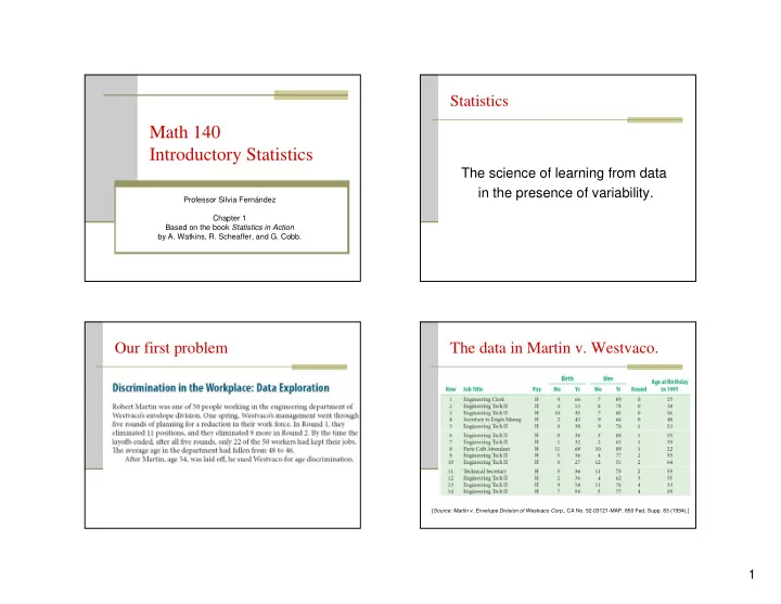
Martin v. Westvaco

Martin: Look at the pattern in the data. All three of the workers

laid off were much older than the average age of all workers. That’s evidence of age discrimination.

Westvaco: Not so fast! You’re looking at only ten people total,

and only three positions were eliminated. Just one small change and the picture would be entirely different. For example, suppose it had been the 25-year-old instead of the 64-year-old who was laid off. Switch the 25 and the 64 and you get a totally different set of averages:

Actual data: 25 33 35 38 48 55 55 55 56 64 Altered data: 25 33 35 38 48 55 55 55 56 64

See! Just one small change and the average age of the three who were laid off is lower than the average age of the others.

47.0 45.0 Altered data 41.4 58.0 Actual data Retained Laid Off

Martin v. Westvaco

Martin: Not so fast, yourself! Of all the possible changes, you

picked the one that is most favorable to your side. If you’d switched one of the 55-year-olds who got laid off with the 55- year-old who kept his or her job, the averages wouldn’t change at all. Why not compare what actually happened with all the possibilities that might have happened?

Westvaco: What do you mean? Martin: Start with the ten workers, treat them all alike, and pick

three at random. Do this over and over, to see what typically happens, and compare the actual data with these results. Then we’ll find out how likely it is that their average age would be 58

• r more.

6

Discussion

• D5. If you pick three of the ten ages at

random, do you think you are likely to get an average age of 58 or more?

• D6. If the probability of getting an average

age of 58 or more turns out to be small, does this favor Martin or Westvaco?

Martin v. Westvaco

Martin: Look at the pattern in the data. All three of the

workers laid off were much older than average.

Westvaco: So what? You could get a result like that

just by chance. If chance alone can account for the pattern, there’s no reason to ask us for any other explanation.

Martin: Of course you could get this result by chance.

Th e question is whether it’s easy or hard to do so. If it’s easy to get an average as large as 58 by drawing at random, I’ll agree that we can’t rule out chance as one possible explanation. But if an average that large is really hard to get from random draws, we agree that it’s not reasonable to say that chance alone accounts for the pattern. Right?

Westvaco: Right

Martin v. Westvaco

Martin: Here are the results of my simulation. If you

look at the three hourly workers laid off in Round 2, the probability of getting an average age of 58 or greater by chance alone is only 5%. And if you do the same computations for the entire engineering department, the probability is a lot lower, about 1%. What do you say to that?

Westvaco: Well . . . I’ll agree that it’s really hard to

get an average age that extreme simply by chance, but that by itself still doesn’t prove discrimination.

Martin: No, but I think it leaves you with some

explaining to do!

Simulation

In our example we can draw 3 of the 10 ages at random and

compute the average. Then repeat this process a large number

• f times to see how likely would be to get 58 or more as the

answer.

Steps in a Simulation:

Random model: Create a model for the chance process

(pieces of paper thoroughly mixed, sequence of random numbers, computer generated random numbers).

Summary Statistic: Calculate it (mean=average in our

example)

Repetition: Repeat a large number of times (1000s) Display the distribution: (Using a dot plot for example) Estimate the Probability: (In our example the proportion of

values that gave 58 or more)

Reach a conclusion: Interpret your results.

7

Simulation Martin Case: Round 2 - Hourly workers

Discussion

• D7. Why must you estimate the probability of

getting an average age of 58 or greater rather than the probability of getting an average age

• f 58?

Discussion

• D8. How unlikely is “too unlikely”? The probability in

the previous activity is in fact exactly equal to 0.05. In a typical court case, a probability of 0.025 or less is required to serve as evidence of discrimination.

• a. Did the Round 2 layoff s of hourly workers in the

Martin case meet the court requirement?

• b. If the probability in the Martin case had been 0.01

instead of 0.05, how would that have changed your conclusions? 0.10 instead of 0.05?

Inference

Inference is a statistical procedure that involves

deciding whether an event can reasonably be attributed to chance or whether you should look for some other explanation.

In the Martin case we used simulation as a device

for inference to determine whether the relatively high average age of the laid-off hourly employees in Round 2 could reasonably be due to chance.

The probability was about 0.05, which was

considered small enough to warrant asking for an explanation from Westvaco but not small enough to present in court as clear evidence of discrimination.

8

Practice

• P4. Suppose three workers were laid off from a set of ten whose

ages were the same as those of the hourly workers in Round 2 in the Martin case. This time, however, the ages of those laid off were 48, 55, and 55. 25 33 35 38 48 55 55 55 56 64

• a. Use the dot plot in Display 1.10 on page 14 to estimate the

probability of getting an average age as large as or larger than that of those laid off in this situation.

• b. What would your conclusion be if Westvaco had laid off

workers of these three ages?

Average age of 3 workers out of 10

45/200=22.5% Actual age average (48+55+55)/3=52.66…

Practice

• At the beginning of Round 1, there were 14 hourly workers. Their ages

were 22, 25, 33, 35, 38, 48, 53, 55, 55, 55, 55, 56, 59, and 64. After the layoffs were complete, the ages of those left were 25, 38, 48, and

• 56. Think about how you would repeat Activity 1.2a using these data.
• a. What is the average age of the ten workers laid off?
• b. Describe a simulation for finding the distribution of the average age of

ten workers laid off at random. (22+33+35+53+55+55+55+55+59+64)/10=48.6 Step 1. Select 10 out of the 14 ages at random and find their average. Step 2. Repeat step 1 many times. (For example, 200 times.) Step 3. Create a dot plot containing the averages obtained from your repetitions.

• c. The results of 200 repetitions from a simulation are shown in Display

1.11. Suppose 10 workers are picked at random for layoff from the 14 hourly workers. Make a rough estimate of the probability of getting, just by chance, the same or larger average age as that of the workers who actually were laid off (from part a).

45 dots out of 200 to the right, corresponding to an average

• f 48.6 or larger.

Estimated probability = 45/200=22.5%

• d. Does this analysis provide evidence in Martin’s favor?

No, a probability of 22.5% is too large to be considered evidence that the actual average may not be due to chance.