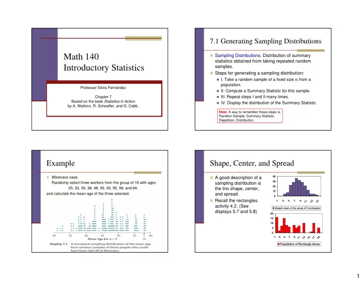
Math 140 Sampling Distributions. Distribution of summary statistics - - PowerPoint PPT Presentation

1

Math 140 Introductory Statistics

Professor Silvia Fernández Chapter 7 Based on the book Statistics in Action by A. Watkins, R. Scheaffer, and G. Cobb.

7.1 Generating Sampling Distributions

Sampling Distributions. Distribution of summary

statistics obtained from taking repeated random samples.

Steps for generating a sampling distribution:

• I. Take a random sample of a fixed size n from a

population.

• II. Compute a Summary Statistic for this sample.
• III. Repeat steps I and II many times.
• IV. Display the distribution of the Summary Statistic.

Note: A way to remember these steps is, Random Sample, Summary Statistic, Repetition, Distribution.

Example

Westvaco case.

Randomly select three workers from the group of 10 with ages 25, 33, 35, 38, 48, 55, 55, 55, 56, and 64, and calculate the mean age of the three selected.

Shape, Center, and Spread

A good description of a

sampling distribution is the trio shape, center, and spread.

Recall the rectangles

activity 4.2. (See displays 5.7 and 5.8)

10 20 30 40 1 3 5 7 9 11 13 15

Sample mean of the areas of 5 rectangles

5 10 15 20 1 3 5 7 9 11 13 15 17 19 Population of Rectangle Areas

2

Shape, Center, and Spread

5 10 15 20 1 3 5 7 9 11 13 15 17 19 Population of Rectangle Areas 10 20 30 40 1 3 5 7 9 11 13 15

Sample mean of the areas of 5 rectangles

• Shape: Irregular
• Center= Mean = μ = 7.41
• Spread =

Standard Deviation = σ = 5.23

• Shape: Normal with a hint of

skew to the right.

• Center= Mean= x = 7.377
• Spread =

Standard Deviation = SE = 2.23

Shape, Center, and Spread

10 20 30 40 1 3 5 7 9 11 13 15

Sample mean of the areas of 5 rectangles

Notes.

The standard deviation of

the sampling distribution is

• ften called the Standard

Error (SE)

Most sample distributions

are nearly normal, we’ll see more about this later.

Values that are in the middle

95% of a random distribution are called Reasonably Likely.

Values that are in the outer

5% of a random distribution are called Rare Events.

• Shape: Normal with a hint of

skew to the right.

• Center= Mean= x = 7.377
• Spread =

Standard Deviation = SE = 2.23

7.2 Sampling distribution of the sample mean.

Example: Population

Sampling distribution of the sample mean for sample sizes 1, 4, 10, 20, and 40.

3

Notation

Size Standard Deviation Mean Sampling Distribution Sample Population

N σ μ n s x SE

x x

• r

σ μ

Properties of The Sampling Distribution of The Sample Mean

The mean of the sampling distribution of equals the mean

• f the population μ:

*The standard deviation of the sampling distribution of ,

also called the standard error of the mean, equals the standard deviation of the population σ divided by the square root of the sample size n:

The Shape of the sampling distribution will be approximately

normal if the population is approximately normal; for other populations, the sampling distribution becomes more normal as n increases. This property is called the Central Limit Theorem.

μ μ =

x

n

x

σ σ =

x

μ

x x

x

σ

*This holds as long as you sample with replacement or your sample size is less than 10% of the population size. (See exercise E30.)

Example 1

Problems usually involve a combination of the

three properties of the Sampling Distribution

• f the Sample Mean, together with what we

learned about the normal distribution.

Example: Average Number of Children

What is the probability that a random sample

• f 20 families in the United States will have

an average of 1.5 children or fewer?

Example 1

Example: Average Number

• f Children

What is the probability that a random sample of 20 families in the United States will have an average of 1.5 children or fewer?

Mean (of population)

μ = 0.873

Standard Deviation

σ =1.095

0.026 4 or more 0.070 3 0.179 2 0.201 1 0.524 Proportion of families, P(x) Number of Children (per family), x

0.1 0.2 0.3 0.4 0.5 0.6 1 2 3 4

4

Example 1

873 . = μ = μx 2448 . 20 095 . 1 = = σ = σ n

x

0.873

Example 1

Find z-score of the value 1.5 So in a random sample of 20

families there is a 99.47% probability that the mean number of children per family will be less than 1.5

873 . = μ = μx 2448 . 20 095 . 1 = = σ = σ n

x

56 . 2 2448 . 873 . 5 . 1 ≈ − = − = − =

x x

x SD mean x z σ μ

9948 . ) 56 . 2 , 99999 ( ≈ − normalcdf

0.873

9948 . ) 2448 . , 873 . , 5 . 1 , 99999 ( OR ≈ − normalcdf

Example 2

Example: Reasonably Likely Averages

What average numbers of children are reasonably likely in a random sample of 20 families?

Recall that the values that are in the middle

95% of a random distribution are called Reasonably Likely.

Note that by calculating the z-scores of 2.5% and 97.5% we find that the Reasonably Likely values are those values within 1.96 standard deviations from the mean. That is, between μ – 1.96 σ and μ + 1.96 σ

Finding Probabilities for Sample Totals

Sometimes situations are stated in terms of the total number in

the sample rather than the average number: “What is the probability that there are 30 or fewer children in a random sample of 20 families in the United States?” You have the choice of two equivalent ways to do this problem.

Method I: Find the equivalent average number of children, x, by

dividing the total number of children, 30, by the sample size, 20: Then you can use the same formulas and procedure as in the previous examples.

Method II: Convert the formulas from the previous examples to

equivalent formulas for the sum, then proceed as in the next example.

5 . 1 20 30 = = x

5

Sampling Distribution

• f the Sum of a Sample

If a random sample of size n is selected with mean μ

and standard deviation σ, then

the mean of the sampling distribution of the sum is the standard error of the sampling distribution of the

sum is

the shape of the sampling distribution will be

approximately normal if the population is approximately normal; for other populations, the sampling distribution becomes more normal as n increases.

μ μ n

sum =

σ σ ⋅ = n

sum

Note: To get the “sum” formulas just multiply by n

Examples 3 and 4

Ex3: The Probability of 25 or fewer Children

What is the probability that a random sample

• f 20 families in the United States will have a

total of 25 children or fewer?

Ex4: Reasonably Likely Totals

In a random sample of 20 families, what total numbers of children are reasonably likely?

Sample Size vs. Population Size

As long as the sample size is a small

percentage (around 10% or less) of the population size, it doesn’t matter much if you sample with or without replacement, and, in fact, the population size will have little effect

• n the statistical analysis.

If the sample size is more than 10% of the

population size then a more complex formula needs to be used for the standard error, we will not do this here since it rarely happens in

• practice. (See Exercise E30.)

7.3 Sampling Distribution

• f the Sample Proportion

You often hear reports of percentages or

proportions: About 60% of automobile drivers in Mississippi use seat belts. (The national average is about 82%.)

To make intelligent decisions based on data

that is reported this way, you must understand the behavior of proportions that arise from random samples.

The properties of sample proportions are

similar to the properties of sample means.

6

The Sample Proportion p-hat

In a certain population we say that p is the proportion

• f the population having a certain property. We say

that p is the proportion of “success” according to our

• property. (e.g. using a seat belt)

Note that p is always a number between 0 and 1. When we select a sample of size n, we calculate the

proportion of successes in our sample by dividing the number of successes by the sample size. We call this the sample proportion and we denote it by p-hat.

n p successes

• f

number size sample successes

• f

number = = ˆ

Simulation (Activity 7.3a)

Choose 10 random

numbers between 1 and

• 10. (use your calculator
• r a random row in the

Table D on page 828)

Count the number of

successes the following way: Numbers between 1 and 6 are successes, 7 to 10 (or 0) are not.

Calculate 10 successes

• f

number ˆ = p

5 10 15 20 25 0.00 0.20 0.40 0.60 0.80 1.00

Computer Simulations

The following diagram shows the exact sampling

distributions of the sample proportion for samples of size 10,20, and 40; when p = 0.6

= 0.6

0.00 0.10 0.20 0.30 0.40 0.50 0.60 0.70 0.80 0.90 1.00 0.00 0.10 0.20 0.30 0.40 0.50 0.6 0.7 0.8 0.9 1 0.00 0.10 0.20 0.30 0.40 0.50 0.6 0.7 0.8 0.9 1

Center and Spread for Sample Proportions

• We can assign successes as

follows:

Non-user of seatbelt 0 User of seat-belt

1

• We then have the following

relative frequency table:

• And by adding the ones we get
• Then we can calculate the

mean of the population as follows

• And in general
• On the other hand we know that

the mean of the sampling distribution of the sample mean is equal to the mean of the population, that is

p 0.6 1 1- 1- p 0.4

In general Relative Frequency Use Seat Belts

x p = = size sample values

• f

sum ˆ

∑

+ = ⋅ = ) 6 . ( 1 ) 4 (. ) (x P x μ p p p x P x = + − = ⋅ = ∑ ) ( 1 ) 1 ( ) ( μ

p

x p

= = = μ μ μ ˆ

7

Center and Spread for Sample Proportions

Similarly we can calculate the standard deviation of

the population as follows and in general

p 0.6 1 1- 1- p 0.4

In general Relative Frequency Use Seat Belts

) 4 . )( 6 . ( ) 4 . 6 . )( 4 . )( 6 . ( 6 . ) 4 . ( 4 . ) 6 . ( 6 . ) 6 . 1 ( 4 . ) 6 . ( ) ( ) (

2 2 2 2 2

= + = + = − + − = = − = ∑ x P x μ σ ) 1 ( ) 1 ( ) 1 ( ) ( ) ( ) (

2 2 2

p p p p p p x P x − = − + − − = = − = ∑ μ σ

Center and Spread for Sample Proportions

On the other hand we know that the standard

deviation of the sampling distribution of the sample mean is equal to the SD of the population divided by the square root of the sample size, that is

n p p n p p n

p x p

) 1 ( ) 1 (

ˆ ˆ

− = − = = = σ σ σ σ

Properties of The Sampling Distribution of The Sample Proportion

• The mean of the sampling distribution of equals the proportion of

successes p:

• The standard deviation of the sampling distribution of , equals the

standard deviation of the population divided by the square root of the sample size n:

• As the sample size gets larger, the shape of the sampling distribution

gets more normal and will be approximately normal if n is large enough.

• As a guideline, if both np and n(1

(1 – p) are at least 10, then using the

normal distribution as an approximation for the shape of the sampling distribution will give reasonably accurate results.

p

p = ˆ

μ n p p

p

) 1 (

ˆ

− = σ

p ˆ

μ

p ˆ p ˆ

p ˆ

σ

Example 5

Drivers in the Northeast and Mid-Atlantic

states had the highest failure rate, 20%, on the GMAC Insurance National Driver’s Test. (They also were the drivers most likely to speed.) [Source: Insurance Journal, www.insurancejournal.com.]

Describe the shape, center, and spread of the

sampling distribution of the proportion of drivers who would fail the test in a random sample of 60 drivers from these states.

What are the reasonably likely proportions of

drivers who would fail the test?

8

More Examples

Example 6. Calculate with p = 0.8 and n =100,

200, 400.

Example 7. Using the Properties to Find Probabilities

About 60% of Mississippians use seat belts. Suppose your class conducts a survey of 40 randomly selected Mississippians.

• a. What is the chance that 75% or more of those

selected wear seat belts?

• b. Would it be quite unusual to find fewer than 25% of

the Mississippians selected wear seat belts?

p ˆ

σ

Finding Probabilities for the Number of Successes

Same as with the sample mean, sometimes problems are stated

in terms of the number of successes rather than the proportion

• f successes. In that case we can again use either of two
• methods. If we use the second method we need to know about

the distribution of the sum of the successes.

• If a random sample of size n is selected from a population with

proportion of success p, then the sampling distribution satisfies:

the shape of the sampling distribution will be approximately

normal if if both np and n(1

(1 – p) are at least 10

np n

p sum

= =

ˆ

μ μ

( )

p np n

p sum

− = ⋅ = 1

ˆ

σ σ

Note: To get the “sum” formulas just multiply by n

Example 8

Probability of 30 or More Wearing Seat Belts

In a random sample of 40 Mississippians, what is the probability that 25 or more use seat belts?

E35

The ethnicity of about 92% of the population of China

is Han Chinese. Suppose you take a random sample

• f 1000 Chinese. [Source: CIA World Factbook.]
• a. Make an accurate sketch, with a scale on the

horizontal axis, of the sampling distribution of the proportion of Han Chinese in your sample.

• b. Make an accurate sketch, with a scale on the

horizontal axis, of the sampling distribution of the number of Han Chinese in your sample.

• c. What is the probability of getting 90% or fewer Han

Chinese in your sample?

• d. What is the probability of getting 925 or more Han

Chinese?

• e. What numbers of Han Chinese would be rare

events? What proportions?

9

Summary: Sampling distributions

success

• f

y probabilit size deviation standard mean Sample Size deviation standard mean Population = = = = = = = p n s x N σ μ n

x x

σ σ μ μ = = mean Sample σ σ μ μ ⋅ = = n n

sum sum

(total) sum Sample

n p p p

p p

) 1 (

ˆ ˆ

− = = proportion Sample σ μ

) 1 ( p np np

sum sum

− = = successes

• f

number Sample σ μ