Math 140 proportions. Introductory Statistics r r p (1 b p (1 b - - PowerPoint PPT Presentation

1

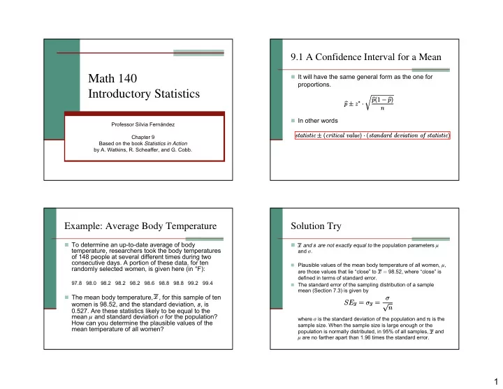
Math 140 Introductory Statistics

Professor Silvia Fernández Chapter 9 Based on the book Statistics in Action by A. Watkins, R. Scheaffer, and G. Cobb.

9.1 A Confidence Interval for a Mean

It will have the same general form as the one for

proportions.

In other words

b p § z¤ ¢ r b p(1 ¡ b p) n b p § z¤ ¢ r b p(1 ¡ b p) n statistic § (critical value) ¢ (standard deviation of statistic) statistic § (critical value) ¢ (standard deviation of statistic)

Example: Average Body Temperature

To determine an up-to-date average of body

temperature, researchers took the body temperatures

• f 148 people at several different times during two

consecutive days. A portion of these data, for ten randomly selected women, is given here (in °F):

97.8 98.0 98.2 98.2 98.2 98.6 98.8 98.8 99.2 99.4

The mean body temperature, x, for this sample of ten

women is 98.52, and the standard deviation, s, is 0.527. Are these statistics likely to be equal to the mean μ and standard deviation σ for the population? How can you determine the plausible values of the mean temperature of all women?

x

Solution Try

x and s are not exactly equal to the population parameters μ

and σ.

Plausible values of the mean body temperature of all women, μ,

are those values that lie “close” to x = 98.52, where “close” is defined in terms of standard error.

The standard error of the sampling distribution of a sample

mean (Section 7.3) is given by where σ is the standard deviation of the population and n is the sample size. When the sample size is large enough or the population is normally distributed, in 95% of all samples, x and μ are no farther apart than 1.96 times the standard error.

SEx = ¾x = ¾ pn SEx = ¾x = ¾ pn

x x x

2

Solution Try (We don’t know σ)

The standard error of the sampling distribution of a sample

mean (Section 7.3) is given by where σ is the standard deviation of the population and n is the sample size. When the sample size is large enough or the population is normally distributed, in 95% of all samples, x and μ are no farther apart than 1.96 times the standard error.

So plausible values of μ lie in the interval We don’t know σ !! (and we shouldn’t expect to know it)

What do we do?

SEx = ¾x = ¾ pn SEx = ¾x = ¾ pn x § 1:96 ¢ ¾ pn or 98:52 § 1:96 ¢ ?? p 10 x § 1:96 ¢ ¾ pn or 98:52 § 1:96 ¢ ?? p 10

x

The effect of estimating σ

In real applications, you almost never know the true

population standard deviation σ

What can we do? Answer: We have to use the sample standard

deviation s as an estimate.

How will making that change—substituting s for σ—

affect your inferences?

Some samples give an estimate that’s too small: s < σ.

Others give an estimate that’s too big: s > σ.

On average the small and large values even out so

that the sampling distribution of s has its center very near σ.

The effect of estimating σ

Although s is about equal to σ on average, it tends to

be smaller than σ more often than it is larger.

This is because the sampling distribution of s is

skewed right. The sampling distribution of s becomes less skewed and more approximately normal as the sample size increases.

50 100 150 200 250 40 80 120 160 200

How to adjust for estimating σ

Estimating the standard deviation does not

affect the center of a confidence interval (the center is at the sample mean x ).

Substituting s for σ does lower the overall

capture rate unless you compensate by increasing the interval widths by replacing z* with a larger value, t*.

Questions: Which value t*? How do we find

it? x

3

Student-Statistician Dialogue

Student: Where does the value of t* come from? Statistician: In principle, you could find it using simulation. Set

up an approximately normal population, take a random sample, compute the mean and standard deviation. Do this thousands of

• times. Then use the results to figure out the value of t* that gives

a 95% capture rate for intervals of the form x– ± t * · s/ .

Student: Wouldn’t that take a lot of work? Statistician: Yes, especially if you went about it by trial and

• error. Fortunately, this work has already been done, long ago. A

statistician, W. S. Gosset (English, 1876–1937), who worked for the Guinness Brewery, actually did this back in 1915. Four years later, the geneticist and statistician R. A. Fisher (English, 1890– 1962) figured out how to find values of t* using probability

• theory. It turns out that the value of t* depends on just two

things—how many observations you have and the capture rate you want.

n s t x / *⋅ ±

Student-Statistician Dialogue

Student: So t* doesn’t depend on the unknown mean or

unknown standard deviation?

Statistician: No it doesn’t, which is very handy because in

practice you don’t know these numbers. Suppose, for example, you have a sample of size n = 5 and you want a 95% interval. Then you can use t* = 2.776 no matter what the values of µ and σ are.

Student: Where did you get that value for t*? Statistician: From a t-table, although I could have gotten it from

a computer. A brief version of the table is shown in Display 9.6. Table B in the Appendix is more complete. The confidence level tells you which column to look in. For example, for a 95% interval, you want a tail area of .025 (half of .05) on either side, so you look in the column headed .025. For the row, you need to know the degrees of freedom, or df for short.

Student-Statistician Dialogue

Student: Degrees of freedom? What’s that? Statistician: There’s a short answer, a longer answer, and a

very long answer. The longer answer will come in E40. The very long answer is for another course. For the moment, here’s the short answer: The degrees of freedom is the number you use for the denominator when you calculate the sample standard

• deviation. So for these confidence intervals, df = n – 1, where n

is your sample size.

• If n = 5, for example, then df = 4 and you look in that row. If you

turn to Table B in the Appendix and look in the row with df = 4 and the column with tail probability 0.025, you’ll find the value 2.776 for t*.

(Better than) Calculator Note

To get t* on your calculator you can use

TInterval and the following values:

x :0 Sx:

n: n

C-Level: Confidence Level

x pn

pn

4

Example: Average Body Temperature

• What is the average body

temperature under normal conditions? Is it the same for both men and women? Medical researchers interested in this question collected data from a large number of men and

• women. Two random samples

from that data, each of size 10, are recorded.

• a. Use a 95% confidence

interval to estimate the mean body temperature of men.

• b. Use a 95% confidence

interval to estimate the mean body temperature of women. 99.4 98.8 99.2 98.6 98.8 98.1 98.8 98.0 98.6 97.9 98.2 97.8 98.2 97.8 98.2 97.5 98.0 97.4 97.8 96.9

Female Male

Body Temperatures (ºF)

Confidence Intervals for a Mean

n s t x ⋅ ± *

A confidence interval for the population

mean, μ, is given by where n is the sample size, x is the sample mean, s is the sample standard deviation, and t* depends on the confidence level desi- red and the degrees of freedom, df = n-1.

x

The Capture Rate

• Similar to Chapter 8, the proportion of intervals of the form

that capture the true value μ of the population mean, is equal to the confidence level. That is a 95% confidence interval will have a 95% capture rate, a 90% confidence interval will have a 90% capture rate, etc.

• This holds as long as

The sample is random (or experimental treatments are randomly

assigned).

The populations is normally distributed. The size of the population is at least 10 times the sample size.

The capture rate will be approximately correct for non-normally distributed populations as long as the sample size is large enough.

n t x σ ⋅ ± *

The Margin of Error.

It is the quantity:

Provided your samples are random, larger samples provide

more information than smaller ones.

As the sample size increases, the margin of error decreases

at a rate proportional to the square root of the sample size.

To cut the margin of error in half, you have to quadruple the

sample size.

To have a margin of error, E, you need a sample size

n larger than

⎟ ⎠ ⎞ ⎜ ⎝ ⎛ ⋅ = E s t n *

2

n s t E ⋅ = *

5

9.2 Significance Test for a Mean μ.

Tests of significance for means have the same general structure as tests for proportions (some details are a bit different). The same four steps:

• 1. Name the test and check the conditions. For a significance

test for a mean three conditions must be met.

the sample was selected at random (or, in the case of an

experiment, treatments were randomly assigned to units)

The sample must look like it came from a normally

distributed population or the sample size must be large

• enough. There is no exact rule for determining whether a

normally distributed population is a reasonable assumption

• r for what constitutes a large enough sample size (more on

this in Section 9.3).

In the case of a sample survey, the population size should

be at least ten times as large as the sample size.

Formal Language of Test Significance

(Components of a Significance Test for a Mean)

• 2. State your hypothesis. The null hypothesis is that

the population mean µ has a particular value µ0.

H0 : The mean μ of the population from which the

sample came is equal to μ0. (μ = μ0) The alternate hypothesis, Ha, can be of three forms:

Ha : The mean μ of the population from which the

sample came is not equal to μ0. (μ ≠ μ0)

Ha : The mean μ of the population from which the

sample came is greater than μ0. (μ > μ0)

Ha : The mean μ of the population from which the

sample came is less than μ0. (μ < μ0)

Formal Language of Test Significance

(Components of a Significance Test for a Mean)

• 3. Compute the test statistic t, find the P-value,

and draw a sketch.

The test statistic is the distance from the sample

mean, to the hypothesized value μ0 measured in standard errors:

The P-value given by your calculator, is the

probability of getting a value of t that is as extreme as

• r even more extreme than the one computed from

the actual sample if the null hypothesis is true.

n s x t / μ − =

Formal Language of Test Significance

(Components of a Significance Test for a Mean)

• 4. Write a conclusion linked to your computations in

the context of the problem.

If you are using fixed-level testing, reject the null

hypothesis if your P-value is smaller than the level of significance, α.

If the P-value is greater than or equal to α, do not

reject the null hypothesis. (If you are not given a value of α, you can assume that is 0.05.)

Write a conclusion that relates to the situation and

includes an interpretation of your P-value.

6

P-Values in your calculator

As always, the P-value is a conditional probability, computed

assuming the null hypothesis is true. It tells the chance of getting a random sample whose value of the test statistic is as extreme as or more extreme than the value computed from the data.

The value of t* depends on the degrees of freedom, so it is a

little more difficult to find the P-value here than it was for the normal case. You can get almost exact P-values from a graphing calculator or computer. Use tcdf(left-endpoint, right-endpoint, df) in your calculator. Where df is one less than the sample size n.

You can only get approximate P-values from a table.

Example: Large Bag of Fries

The statistics class at the University of Wisconsin–Stevens Point estimated the average mass of a large bag of french fries at McDonald’s. They bought 30 bags during two different half-hour periods on two consecutive days at the same McDonald’s and weighed the fries. McDonald’s “target value” for the mass of a large order of fries was 171 g. Is there evidence that this McDonald’s wasn’t meeting that target?

Example: One-Sided P-Values

A book about different colleges reports that

the mean time students at a particular university study each week is 1015 minutes. A dean says she believes the mean is greater than 1015 minutes. To test her claim, she takes a random sample of 64 students and finds the sample mean is 1050 minutes, with standard deviation 150 minutes. Is this strong evidence in favor of her claim?

Example: Distance from the Sun

“Earth is 93 million miles from the Sun.” You

have probably heard or read that often. But is it true? The table on the right shows 15 measurements made of the average distance between Earth and the Sun (called the Astronomical Unit, abbreviated A.U.), including Newcomb’s original measurement from 1895. Use these data to test the hypothesis that they are consistent with the true mean A.U. being 93 million miles. Use a .05 significance level.

92.81 92.96 92.96 92.92 92.88 92.87 92.91 92.98 92.84 92.91 93.00 92.87 92.91 92.83 93.28

Astronomical Unit (millions of miles)

7

9.4 Inference for the Difference Between Two Means

Most scientific studies involve comparisons. For

example, for purposes of studying pesticide levels in a river, does it make a difference whether you take water samples at mid-depth, near the bottom, or at the surface of the river? Do special exercises help babies learn to walk sooner?

Inference about comparisons is more often used in

scientific investigations than is inference about a single parameter.

Almost all experiments are comparative in nature.

The study of inference for differences, then, is fundamental to statistical applications.

Example

The Wolf River in Tennessee

flows past an abandoned site

• nce used by the pesticide

industry for dumping wastes, including hexachlorobenzene (chlordane), aldrin, and dieldren.

These highly toxic organic

compounds can cause various cancers and birth defects. The standard method to test whether these poisons are present in a river is to take samples at six- tenths depth, that is, six-tenths

• f the way from the surface to

the bottom.

• Unfortunately, there are good

reasons to worry that six-tenths is the wrong depth. The organic compounds in question don’t have the same density as water, and their molecules tend to stick to particles of sediment. Both these facts suggest you’d be likely to find higher concentrations near the bottom than near mid-depth.

Example

• The Wolf River in Tennessee flows past

an abandoned site once used by the pesticide industry for dumping wastes, including hexachlorobenzene (chlordane), aldrin, and dieldren. These highly toxic organic compounds can cause various cancers and birth defects. The standard method to test whether these poisons are present in a river is to take samples at six-tenths depth, that is, six-tenths of the way from the surface to the bottom. Unfortunately, there are good reasons to worry that six-tenths is the wrong depth. The organic compounds in question don’t have the same density as water, and their molecules tend to stick to particles of sediment. Both these facts suggest you’d be likely to find higher concentrations near the bottom than near mid-depth. Concentration of Aldrin in nanograms per liter

Confidence Interval for the Difference Between Two Means

As usual the general form looks like: Here: So the confidence interval is given by: We need to verify three conditions:

Samples have been randomly and independently selected from two

different populations (or two treatments were randomly assigned).

The two populations are approximately normally distributed or the

sample sizes are large enough.

In case of surveys, the population size should be at leastten times

larger than the sample size for both samples.

estimate)

• f

estimate SE t ( *⋅ ±

2 2 2 1 2 1 2 1 2 1

, n s n s s SE x x

x x

+ = = − =

−

estimate

• f

and estimate

2 2 2 1 2 1 ) 2 1

* ( n s n s z x x + ⋅ ± −

8

Confidence Interval for the Difference Between Two Means.

Here is highly recommended to use a

calculator because finding t* is complicated because it depends on df, and for the difference of two means we have that

) 1 /( ) 1 /(

2 2 2 2 1 1 2 1 2 2 2 1 2 1

2 2 2

− ⎟ ⎟ ⎠ ⎞ ⎜ ⎜ ⎝ ⎛ + − ⎟ ⎟ ⎠ ⎞ ⎜ ⎜ ⎝ ⎛ ⎟ ⎟ ⎠ ⎞ ⎜ ⎜ ⎝ ⎛ + = n n s n n s n s n s df

Example

Construct a 95% confidence

interval for the difference between the mean bottom measurement of aldrin in the Wolf River and the mean mid-depth measurement.

Concentration of Aldrin in nanograms per liter

Example: Walking Babies

• Some babies start walking well before they are a year old, whereas others

still haven’t taken their first unassisted steps at 18 months or even later. The data in the Display come from an experiment designed to see whether a program of special walking and placing exercises for 12 minutes each day could speed up the process of learning to walk. In all, 23 male infants (and their parents) took part in the study and were randomly assigned either to the special exercise group or to one of three control groups.

• The effects of special exercises to speed up infant walking were isolated

with three different control groups. The data is shown.

• Use these data to find a 95% confidence interval estimate of the difference

between mean walking times for the special exercises group and the exercise control group if all babies could have had each treatment.

Significance Tests for the Difference

• f Two Means ( σ1 and σ2 unknown).

See page 625 in your book.

9

Example: Wolf River

You’ve been given the

responsibility to analyze the Wolf River data to test whether the true mean aldrin concentrations at the bottom and mid-depth might differ. That is, you want to set up a test of significance for the difference between two population means based on data from independent random

• samples. Use α = 0.10.

Concentration of Aldrin in nanograms per liter

9.3 How Large a Sample? The 15/40 rule for t-procedures.

If your sample size is less than 15: Be very careful. Your data

• r transformed data must look like they came from a normal

distribution—little skewness, no outliers.

If your sample size is between 15 and 40: Proceed with

caution.

Strongly skewed distributions should be transformed to a

scale that makes them more nearly symmetric before using the t-procedures.

If you have gross outliers, a transformation may be in order.

If you don’t transform or if the outliers remain even after a change of scale, do two versions of your test or interval, one with and one without the outliers.

• Don’t rely on any conclusions that depend on whether you

include the outliers.

9.3 How Large a Sample? The 15/40 rule for t-procedures.

If your sample size is over 40: You’re in good shape. Your

sample size is large enough that skewness will not reduce capture rates or alter significance levels enough to matter.

Still, if your sample shows strong skewness, it is worth

asking whether a change of scale would make the usual summary statistics (especially the standard deviation) more

• meaningful. Even though outliers may not have much effect
• n capture rates or significance levels, you should still check

by doing two versions of your t-procedure.

Examples of Transformations

10

Examples of Transformations

Apply Logarithm to the data

Significance Tests Various Examples

• 1. A job placement director claims that the average starting

salary for nurses is $24,000. A sample of 10 nurses' salaries has a mean of $23,450 and a standard deviation of $400. Is there enough evidence to reject the director's claim at α=0.05.

• 2. A statistician read that at least 77% of the population oppose

replacing $1 bills with $1 coins. To see if this claim is valid, the statistician selected a sample of 80 people and found that 55 were opposed to replacing the $1 bills. At α=0.01, test the claim that at least 77% of the population are opposed to the change.

• 3. A researcher reports that the average salary of an assistant

professor is more than $42,000. A sample of 30 assistant professors has a mean salary of $43260 and a standard deviation of $5230. At α=0.05, test the claim that assistant professors earn more than $42,000 a year.

Significance Tests Various Examples

• 4. In a sample of 200 surgeons, 15% thought the government

should control health care. In a sample of 200 general practitioners, 21% felt the same way. At α=0.01, is there a difference in the proportions?

• 5. The average size of a farm in Indiana County, Pennsylvania,

is 191 acres. The average size of a farm in Greene County, Pennsylvania, is 199 acres. Assume the data were obtained from two samples with standard deviations 38 and 12 acres, respectively, and sample sizes of 8 and 10, respectively. Can it be concluded at α=0.05 that the average size of the farms in the two counties is different? Assume the populations are normally distributed.

• 6. A survey found that the average hotel room rate in New

Orleans is $88.42 and the average room rate in Phoenix is $80.61. Assume that the data were obtained from two samples

• f 50 hotels each and that the standard deviations of these

samples were $5.62 and $4.83 for New Orleans and Phoenix,

• respectively. At α=0.03, can it be concluded that there is a

significant difference in the rates?