- masses M , stiffness K - modes Physical linear dynamic model. - - PowerPoint PPT Presentation

Statistical Approaches to Industrial Monitoring Problems - Fault Detection and Isolation

• M. Basseville, Q. Zhang, A. Benveniste

IRISA (CNRS and INRIA), Rennes, France Three examples Design of the algorithms : heuristics Design of the algorithms : theory Design of the algorithms : back to the examples

1

Introduction Signal processing and on-board monitoring

Early detection of slight deviations with respect to a characterization of the system in usual working conditions ⇓ Condition-based maintenance, predictive maintenance

2

Three examples

Structural vibration monitoring Physical linear dynamic model. Combustion set of gas turbines Semi-physical non-linear static model. Catalytic converter of an automobile Semi-physical non-linear dynamic model.

3

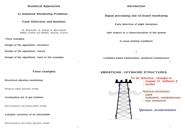
To be detected : changes in VIBRATIONS : OFFSHORE STRUCTURES

• swell

Sensors: accelerometers

• turbulent, nonstationary

Natural excitation :

• non measured
• masses M, stiffness K
• modes

4

To be detected : changes in Ambiant excitation: VIBRATIONS : ROTATING MACHINES Sensors: accelerometers (on the bearings!)

• load unbalancing, frictions, steam
• non stationary, non measured
• modes
• masses M, stiffness K

5

Structure

OK? Detection, diagnostics :

ζ = 0? (physical, linear, dynamic model)

Which M, K failed? Changed modes?

ζ shows if the model still fits the data

VIBRATIONS: MONITORING SCHEME

Y

(not measured)

V

nonstationary

6

COMBUSTION : GAS TURBINES chambers Combustion Turbine Sensors : thermocouples at the exhaust To be detected : changes in burners and turbine Compressor

7

chambers Combustion Detection, diagnostics : static model) Turbine (Semi-physical, nonlinear,

ζ = 0? Y Did the turbine fail? OK? Which chamber? COMBUSTION : MONITORING SCHEME ζ shows if the model still fits the data V U

8

AUTOMOBILE : DEPOLLUTION SYSTEM catalytic converter, front λ oxygen sensors λ λ To be diagnosed (OBD2 norm) : Catalytic converter Sensors : λ oxygen gauges Engine, and control exhaust

9

DEPOLLUTION : MONITORING SCHEME

dynamic model) nonlinear,

V

Oxygen (Semi-physical,

(semi-phys., nonlinear, dynamic model)

Cata.converter Controlled engine (Simplified model)

Z

sensor

Y2 Y1

Detection, diagnostics ζ = 0?

Converter? Sensor? OK?

10

Design of the algorithms : heuristics

(Model validation)

Modeling and identification Monitoring Reduction to a universal problem

11

On-Board Detection : don’t re-identify!

NEW distance data-to-model REFERENCE NEW DATA REFERENCE model-to-model distance

12

Monitored system U

• bserved
• bserved

U, Y V, Z not V Y = M(θ, U) θ : parameter Y Z θ0 Modeling and identification θ0 = arg minθ Σk (Yk − M(θ, Uk))2

• r θ :

Σk C(Yk, M(θ0, Uk)) = 0

13

V U Monitored system Y Z ζ(θ, U, Y ) ∆ =

∂ ∂θ Σk (Yk − M(θ, Uk))2

• r: ζ(θ, U, Y ) ∆

= Σk C(Yk, M(θ, Uk)) Y = M(θ0, U) ζ(θ0, U, Y ) = 0? Monitoring

14

Reduction to a universal problem

ζN

∆

= ζ

• θ0, YN

1

• =

0 ? Local approach Test H0 : θ = θ0 against H1 : θ = θ0 + δθ √ N ζN ∼ N (0, Σ(θ0)) ζN ∼ N (M(θ0) δθ, Σ(θ0)) χ2 in ζN Noises and uncertainty on θ0 taken into account.

15

Design of the algorithms : theory

Local approach : likelihood Local approach : other estimating/monitoring functions

16

Local approach : likelihood

Log-likelihood function ln pθ(YN

1 ) = N

• k=1 ln pθ(Yk|Yk−1

1

) Efficient score ζN(θ0) ∆ = 1 √ N ∂ ln pθ(YN

1 )

∂θ

• θ=θ0

= 1 √ N

N

• k=1 . . .

Fisher information matrix I(θ) ∆ = lim

N→∞ IN(θ),

IN(θ) ∆ = cov ζN(θ) = − 1 N Eθ ∂2 ln pθ(YN

1 )

∂θ2

17

Second order Taylor expansion of the log-likelihood ratio θ = θ0 + δθ √ N SN(θ0, θ) ∆ = ln pθ(YN

1 )

pθ0(YN

1 ) ≈ δθT ζN(θ0) − 1

2 δθT I(θ0) δθ Eθ0 SN ≈ − 1 2 δθT I(θ0) δθ Eθ SN ≈ + 1 2 δθT I(θ0) δθ ≈ − Eθ0 SN covθ0 SN ≈ δθT I(θ0) δθ ≈ covθ SN

18

First order Taylor expansion of the efficient score ζN(θ) ≈ ζN(θ0) + 1 N ∂2 ln pθ(YN

1 )

∂θ2

• θ=θ0

δθ Eθ0 ζN(θ) ≈ − I(θ0) δθ Efficient score = ML estimating function Eθ0 ζN(θ) = 0 ⇐ ⇒ θ = θ0 Caution : Efficient score = innovation !

19

Example : Gaussian scalar AR process Yk =

p

• i=1 ai Yk−i + Ek,

θT = ( a1 . . . ap ) ζN(θ) = 1 √ N 1 σ2

N

• k=1 Y−

k−1,p εk(θ)

I(θ) = 1 σ2 Tp Efficient score ζ : vector-valued function Innovation ε : scalar function

20

Hypotheses testing - CLT

Locally Asymptotic Normal (LAN) family (Le Cam, 1960) SN(θ0, θN)

∆

= ln pθN(YN

1 )

pθ(YN

1 )

≈ δθT ζN(θ0) − 1

2 δθT IN(θ0) δθ + αN(θ0, YN 1 , δθ)

ζN(θ0) → N(0, I(θ0)) αN → 0 a.s. under H0 Examples : i.i.d. variables, stationary Gaussian processes, stationary Markov processes.

21

CLT in LAN families

(i.i.d. variables, stationary Gaussian processes, stationary Markov processes) SN(θ0, θ) →

                    

N( − 1

2 δθT I(θ0) δθ,

δθT I(θ0) δθ) under Pθ0 N( + 1

2 δθT I(θ0) δθ,

δθT I(θ0) δθ) under Pθ0+ δθ

√ N

ζN(θ0) →

                  

N( 0, I(θ0)) under Pθ0 N( I(θ0) δθ, I(θ0)) under Pθ0+ δθ

√ N

ζN is asymptotically a sufficient statistics.

22

Asymptotically optimum tests for composite hypotheses Asymptotically equivalent problems : (1) : P = {Pθ}θ∈Θ⊂Rℓ LAN YN

1 ,

N → ∞ H0 = {θ ∈ Θ0}, H1 = {θ ∈ Θ1}, Θi = θ0 + Γi √ N (2) : ζ ∼ N(Υ, I−1(θ0)) H0 = {Υ ∈ Γ0}, H1 = {Υ ∈ Γ1}

23

Asymptotically equivalent and UMP tests (Kushnir-Pinski, 1971; Nikiforov, 1982)

1 O( ) N

supθ∈Θ1 pθ(YN

1 )

supθ∈Θ0 pθ(YN

1 )

≥ λ pˆ

θ(YN 1 )

pθ0(YN

1 )

≥ λ N (ˆ θ − θ0)T I(θ0) (ˆ θ − θ0) ≥ λ ζT

N(θ0) I−1(θ0) ζN(θ0) ≥ λ

24

Local approach : other estimating functions

Quasi-score ζN(θ0) = 1 √ N

N

• k=1 H(θ0, Yk)

Estimating function Eθ0 H(θ, Yk) = 0 ⇐ ⇒ θ = θ0 Mean deviation M(θ0) ∆ = − Eθ0 ∂ ∂θ H(θ, Yk)

• θ=θ0

25

Computation of the mean deviation M(θ0)

∆

= − Eθ0 ∂ ∂θ H(θ, Yk)

• θ=θ0

= − ∂ ∂θ Eθ0 H(θ, Yk)

• θ=θ0

= + ∂ ∂θ Eθ H(θ0, Yk)

• θ=θ0

= covθ0

• ζN(θ0), ζML

N (θ0)

• (i.i.d. case)

26

First order Taylor expansion of a quasi-score θ = θ0 + δθ √ N ζN(θ) ≈ ζN(θ0)

• +

√ N 1 N

    

N

• k=1

∂ ∂θ H(θ, Yk)

• θ=θ0

    

• δθ

√ N |

under CLT

| ↓ θ0 |

under LLN

| ↓ θ0 N(0, Σ(θ0)) Eθ0 ∂ ∂θ H(θ, Yk)

• θ=θ0
• = − M(θ0)

27

Estimation efficiency and covariance of estimating fct √ N

ˆ

θN − θ0

• ≈ −

    Eθ0

∂ ∂θ H(θ, Yk)

• θ=θ0

    

−1

• ζN(θ0)

M(θ0)−1 Hence cov

ˆ

θN − θ0

• =
• MT(θ0) Σ−1(θ0) M(θ0)

−1

28

Quasi score - CLT (McLeish, 1977; Heyde, 1989; Delyon and Juditsky, 1997) ζN(θ0) →

                  

N( 0, Σ(θ0)) under Pθ0 N( M(θ0) δθ, Σ(θ0)) under Pθ0+ δθ

√ N

Tests for composite hypotheses (Basawa, 1985; Benveniste et al., 1987) ζT

N

Σ−1 M

• MT Σ−1 M

−1 MT Σ−1

• ζN

≥ λ I−1 χ2-test invariant w.r.t. pre-multiplication of H (and thus ζ) by an invertible matrix gain.

29

Design of the algorithms : back to the examples

Vibrations Gas turbines Catalytic converter

30

Structural vibration monitoring

              

M ¨ Zt + C ˙ Zt + KZt = Et (Mµ2 + Cµ + K)Ψµ = 0 Yt = LZt ψµ = LΨµ

              

Xk+1 = F Xk + Wk F ϕλ = λ ϕλ Yk = HXk eτµ = λ, ψµ = Hϕλ Yk =

p

• i=1 Ai Yk−i +

q

• j=0 Bj(k) Vk−j

H F p =

p

• i=1 Ai H F p−i

Monitor AR part, with nonstationary MA part. Modal changes not visible on spectra (1%). Likelihood : no hope !

31

Eigenstructure monitoring

                

Xk+1 = F Xk + Wk F ϕλ = λ ϕλ Yk = HXk Φλ

∆

= H ϕλ Canonical system parameter θ ∆ =

   

Λ vec Φ

    ,

Op+1(θ) =

           

Φ Φ∆ . . . Φ∆p

           

System parameter characterization Hp+1,q and Op+1(θ) have the same left kernel space

32

• 1. Input-output (IV-based) monitoring functions :

(Roug´ ee, 1985)

• AT

−Ir

• H0

p+1,q = 0

                                        

AT ∆ = ( Ap . . . A1 ),

• Hp+1,q =

            

ˆ R0 ˆ R1 . . . ˆ Rq−1 ˆ R1 . . . . . . . . . . . . . . . . . . . . . ˆ Rp . . . . . . ˆ Rp+q−1

            

• AT (θ0) −Ir
• Op+1(θ0) = 0

ζN(θ0) = √ N vec

• ( AT (θ0) −Ir )
• Hp+1,q
• Hp+1,q =

1 N − p − q + 1

N−p

• k=q Y+

k,p+1 Y− k,q T

33

• 2. Subspace-based monitoring functions :

(Abdelghani et al., 1996) SVD of W1

• H0

p+1,q W T 2

                

ST (θ) W1

• H0

p+1,q W T 2 = 0

ST S = Is, ST W1 Op+1(θ) = 0 ζN(θ0) = √ N vec

• ST (θ0) W1
• Hp+1,q W T

2

• Hp+1,q =

1 N − p − q + 1

N−p

• k=q Y+

k,p+1 Y− k,q T

34

Experimental results

– Simulated and real data (offshore platform, alternator): – Detect < 1% frequency changes – Detect changes mainly in modal shapes – In the LMS modal analysis software environment: current experiments on several laboratory experimental se- tups and international benchmarks

35

Combustion set of gas turbines

yj = f(U)

10

• i=1 αi g(φj − h(U) − β)

(1 ≤ j ≤ 18) θ ∆ =

α1 . . . α10 β T

Yk(θ) ∆ =

y1 . . . y18 T (k)

Noisy outputs Y and inputs U : biased reference θ0. Identification bias is not an obstacle to monitoring! (Zhang, 1992)

36

LS-score H(θ, Yk, Uk) = −

   

∂ǫk(θ) ∂θ

   

T

ǫk(θ) ǫk(θ) = Yk − Yk(θ) Bias-adjusted estimating function ˆ h0 = 1 N

N

• k=1 H(θ0, Y 0

k , U0 k)

ζN(θ0) = 1 √ N

N

• k=1
• H(θ0, Yk, Uk) − ˆ

h0

• 37

Robustness w.r.t. operating conditions : shape of the hypotheses! (Mathis, 1994)

38

Experimental results

– Simulated and real data (a turbine operating during several months) – Two algorithms tuned and implemented differently :

• ne on-line: for large sudden drops in temperatures,

the other off-line: for smaller and slower drops – Robustness improved using confidence ellipsoids – Correct diagnostics

39

Catalytic converter and oxygen sensor of an automobile

              

˙ X = f(θ, X, U) Y = g(θ, X, U)

                        

δXk = f(θ, Xk, Uk) Yk = g(θ, Xk, Uk) + ε(Y )

k

Unknown input U; highly nonlinear functions f, g.

40

• 1. Full state observer and LS-prediction-score :

H(θ, Yk

1 , Uk 1 ) =

     

∂ ˆ Yk|k−1(θ) ∂θ

     

T

• Yk − ˆ

Yk|k−1(θ)

• 

               

ˆ Xk|k−1 = ˆ f(θ, ˆ Xk−1|k−2, Yk−1, Uk−1) ˆ Yk|k−1(θ) = g(θ, ˆ Xk|k−1, Uk−1) ∂ ˆ Yk|k−1(θ) ∂θ solution of a differential system.

41

• 2. Input-output description and LS-score : (Zhang, 1996)

F (θ, Yk, Uk, δ) = ε(F )

k

H(θ, Yk, Uk, δ) = −

   ∂F (θ, Yk, Uk, δ)

∂θ

   

T

F (θ, Yk, Uk, δ) F (θ, Yk, Uk, δ) = P (Yk, Uk, δ) θ − Q(Yk, Uk, δ) 2 H(θ, Yk, Uk, δ) = − P T (Yk, Uk, δ) P (Yk, Uk, δ) θ + P T(Yk, Uk, δ) Q(Yk, Uk, δ)

42

Experimental results

– Combined LS-score and observer : Simulated and real data – catalytic converter and front oxygen sensor; – some subsystems of a nuclear power plant; – some subsystems of a thermal plant. – Combined LS-score and input-output equations : – some subsystems of a nuclear power plant.

43

Statistical approaches to isolation

ζ ∼ N(M η, ¯ Σ ¯ ΣT ), η =

    ηa

ηb

    ,

M =

Ma Mb

• ,

pηa,ηb(ζ)

Decide between ηa = 0 and ηa = 0; ηb unknown

I = MT Σ−1 M ∆ =

    Iaa Iab

Iba Ibb

   

I∗−1

a

: upper-left term of I−1 ; I∗

a = Iaa − Iab I−1 bb Iba

44

Statistical projection (sensitivity)

2 ln maxηa pηa,0(ζ) p0,0(ζ) = ζT

a I−1 aa ζa ,

ζa : partial score

Statistical rejection (minmax)

2 ln maxηa,ηb pηa,ηb(ζ) maxηb p0,ηb(ζ) = ζ∗T

a

I∗ −1

a

ζ∗

a ,

ζ∗

a : effective score

ζ∗

a = ζa − Iab I−1 bb ζb

regression of partial score on nuisance score (Neyman,1954). Optimality (Spjotvoll, 1971; Mathis, 1994).

45

On-Board Diagnostics : don’t solve the inverse problem!

complex, not identifiable DATA simple, identifiable REFERENCE (BLACK-BOX) MODEL OF PHYSICAL SYSTEM black-box diagnostics physical diagnostics

46

‘Black-box’ diagnostics : sensitivity

δθi = Ji δφi, dim φ = dim θ

‘Physical’ diagnostics : sensitivity with model reduction

δθi = Ji δΦi, dim Φ ≫ dim θ Aggregate the δθi with the metric of the χ2-test.

47

Optimal sensor location

Maximize the power of the detection algorithms : Trace (MT Σ−1 M) Physical model necessary, ‘compensate’ for the number of d.o.f. of χ2 tests. Two possible uses : – For a given set of faults : how many sensors, and where? – For a given sensor pool : which faults are detectable?

Fault detectability

48

Conclusion

Actual and potential benefits of statistical local approach Question: quasi-scores for (complex) state-space models?

49