M Z ( s ) + C Z ( s ) + K Z ( s ) = ( s ) FE - - PowerPoint PPT Presentation

SLIDE 1

Handling the temperature effect in vibration monitoring of civil structures: a combined subspace-based and nuisance rejection approach

´ Etienne Balm` es MssMat, Ecole Centrale Paris, France Mich` ele Basseville, Laurent Mevel, Houssein Nasser IRISA (CNRS & INRIA & Univ.), Rennes, France National Computer & Security project Constructif houssein.nasser@irisa.fr -- http://www.irisa.fr/sisthem/

1

Introduction

• Usefulness of global vibration-based SHM methods
• Limitations due to temperature effects on the dynamics
• f civil engineering structures
• Wanted: discriminate between changes in modal parameters

due to damages and changes due to temperature effects

• A statistical subspace-based damage detection algorithm:

null space of a matrix built on reference modes/modeshapes at a known temperature

• Proposed solution to temperature handling:

no temperature measurement, thermal effect modeling, statistical nuisance rejection

2

Content

Parametric subspace-based damage detection The temperature effect - Examples The temperature effect - Modeling The temperature effect - Rejection Experimental results Conclusion

3

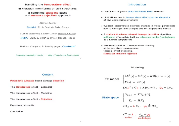
Modeling FE model:

                  

M ¨ Z(s) + C ˙ Z(s) + KZ(s) = ν(s) Y (s) = LZ(s) (Mµ2 + Cµ + K)φµ = 0 , ψµ = Lφµ State space:

                  

Xk+1 = F Xk + Vk Yk = HXk F Φλ = λ Φλ , ϕλ

∆

= HΦλ eτµ = λ

• modes

, ψµ = ϕλ

• modeshapes

4

SLIDE 2

Parametric subspace-based damage detection

                    

Xk+1 = F Xk + Vk F Φλ = λ Φλ Yk = H Xk ϕλ

∆

= H Φλ Ri

∆

= E

 Yk Y T

k−i

  ,

H

∆

=

              

R0 R1 R2 . . . R1 R2 R3 . . . R2 R3 R4 . . . . . . . . . ... . . .

              

Ri = H F i G = ⇒ H = O C

O ∆ =

        

H HF HF 2 . . .

        

, C ∆ =

G

F G F 2G . . .

• G ∆

= E

• Xk Y T

k

• H −

→ O − → (H, F ) − → (λ, φλ)

5

Canonical parameter : θ ∆ =

   

Λ vec Φ

   

modes mode shapes

Observability in modal basis : Op+1(θ) =

        

Φ Φ∆ . . . Φ∆p

        

θ0 : reference parameter for safe structure Left null space: ST S = Is, ST Op+1(θ0) = 0 Yk: N-size sample of new measurements Residual for SHM: ζN(θ0) ∆ = √ N vec( ST (θ0) ˆ H )

J (θ0): sensitivity of ζ w.r.t. modal changes; Σ(θ0): covariance

χ2-test: ζT

N Σ−1 J (J T Σ−1 J )−1 J T Σ−1ζN

≥ h

6

Focussed monitoring

Fisher information F(θ0) ∆ = J (θ0)T Σ(θ0)−1 J (θ0) θ =

    θa

θb

    , J = (Ja Jb), F =     Faa Fab

Fba Fbb

    =     J T

a Σ−1Ja J T a Σ−1Jb

J T

b Σ−1Ja J T b Σ−1Jb

   

F⋆

a ∆

= Faa − Fab F−1

bb

Fba

Sensitivity approach - Partial residual ˜ ζa ∆ = J T

a Σ−1 ζ,

˜ χ2

a ∆

= ˜ ζT

a F−1 aa ˜

ζa Min-max approach - Robust residual ζ⋆

a ∆

= ˜ ζa − Fab F−1

bb

˜ ζb, χ⋆ 2

a

= ζ⋆T

a

F⋆ −1

a

ζ⋆

a

7

The temperature effect - Example 1 Z24 bridge

• A benchmark of the BRITE/EURAM project SIMCES and of

the European COST action F3

• Response to traffic excitation under the bridge

measured over one year in 139 points

• Two damage scenarios (DS1 and DS2):

pier settlements of 20mm and 80mm.

8

SLIDE 3

Identified first four natural frequencies / Test values (Results with four sensors) Mode 1 2 3 4 χ2 Undamaged Freq.(Hz) 3.88 5.01 9.80 10.30 8.80 · 10e2 Damaged (1) Freq.(Hz) 3.87 5.06 9.79 10.32 8.00 · 10e5 Damaged (2) Freq.(Hz) 3.76 4.93 9.74 10.25 3.96 · 10e6

9

Evolution of the test values over nine months (log-scale). Distribution of the test values for each of the nine months.

10

The temperature effect - Example 2 Simulated bridge deck

Finite elements toolbox OpenFEM (with Matlab or Scilab). 60 m span, 9600 volume elements, 13668 nodes. Temperature variations: either a uniform temperature elevation

• r a linear variation with z.

Linear thermal field (Left) and induced axial stress (Right). The warmer deck expands while the cooler bottom contracts.

11

−1 −2 −3 −4 −5 −6 −7 −8 1.685 1.69 1.695 1.7 1.705 1.71 1.715 1.72 ∆T° Frequency

safe damaged

Decreasing temperature effect on the first frequency.

−1 −2 −3 −4 −5 −6 −7 −8 500 1000 1500 2000 2500 3000 3500 4000 ∆T° χ2

safe damaged

Partial χ2-test values. Safe and damaged

12

SLIDE 4

The temperature effect - Modeling

• Thermal field → materials expansion → thermal stress field.
• Temperature modification = external load.
• Static equilibrium under thermal loading ↔ pre-stress.
• Stiffness K, and thus modal frequencies, affected.

Mass M and damping C assumed not affected.

• Assuming thermal loads inducing small perturbations:

stiffness = linear function of the thermal field T (x).

• If T (x) = linear combination of constant thermal fields,

temperature effect on K: K = K0 + KT

∆

= K0 +

• i αi KT,i

13

Computing the residual sensitivity w.r.t. T

Small deviations E(ζN) = J (θ0) δθ + JT δT, JT

∆

= J (θ0) JθT JθT involves computing δµ and δφ for δK = KT,i, δM = δC = 0, based on the differentiation of: (Mµ2 + Cµ + K)φµ = 0 that is: δµ = − φT (µ2 δM + µ δC + δK) φ φT (2 µ M + C) φ and (µ2 M +µ C +K) δφ = − δµ (2 µ M +C) φ−(µ2 δM +µ δC +δK) φ with φT δφ = 0.

14

The temperature effect - Rejection

• θ0 : reference modal parameter for safe structure

Compute the null space S(θ0), the sensitivities J (θ0) and JT , the covariance Σ(θ0) and Fisher matrix F ∆ = F(θ0, T )

• Yk: N-size sample of new measurements
• Compute the residual ζN(θ0) ∆

= √ N vec( ST (θ0) ˆ H )

• Compute the robust residual ζ⋆

θ0 ∆

= ˜ ζθ0 − Fθ0,T F−1

T,T ˜

ζT

• Compute the χ2-test : ζ⋆

θ0 T F⋆ −1 θ0

ζ⋆

θ0

15

Implementation issues

• Compute the key matrices:

sensitivities J (θ0) and JT and covariance Σ

• n a long data sample for the safe structure.

In case of nonstationary excitation, computing Σ

• n current data might be preferable.
• Σ computed with QR (Zhang, 2003).

Null space S computed with QR (Nasser, 2006).

16

SLIDE 5

Example - Back to the simulated bridge deck

1 2 3 4 5 6 7 8 1.67 1.675 1.68 1.685 1.69 1.695 1.7 1.705 ∆T° Frequency

safe damaged

Increasing temperature effect on the first frequency.

1 2 3 4 5 6 7 8 2 4 6 8 10 12 14 16 18 x 104 ∆T° χ2

safe without rejection damaged without rejection safe with rejection damaged with rejection

Global (dotted) and minmax (solid) χ2-test values. Minmax operating range: 8 C × 2 Safe and damaged

17

Conclusion

Temperature effect in vibration-based SHM Statistical parametric model-based approach Subspace-based damage detection algorithm Local rejection of the temperature seen as nuisance Example: simulated bridge deck Ongoing: empirical null space merging data at # temperatures, analytical temperature-adjusted null space Future: in-operation examples, extension to 3D temperature fields, thermal model parameterization

18