LYR M&E Plan Spatial Structure CAN YOU SEE ME? A populations - - PowerPoint PPT Presentation

2D PHYSICAL HABITAT ANALYSIS

LYR M&E Plan Spatial Structure

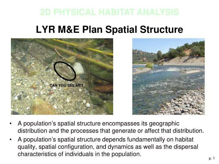
• A population’s spatial structure encompasses its geographic

distribution and the processes that generate or affect that distribution.

• A population’s spatial structure depends fundamentally on habitat

quality, spatial configuration, and dynamics as well as the dispersal characteristics of individuals in the population.

• p. 1

CAN YOU SEE ME?

2D PHYSICAL HABITAT ANALYSIS

Physical Habitat

• Location with measurable, characteristic attributes where
• rganisms perform a designated ecological function.
• Attributes stem from interaction among hydrology,

hydraulics, and geomorphology

• Depth, velocity, substrate, temperature, cover are the most

common attributes used.

• Microhabitat- point-scale locations
• Mesohabitat- patches at the 0.1-10 channel-width scale
• p. 2

2D PHYSICAL HABITAT ANALYSIS

Physical Habitat Performance Indicators

• [Species X lifestage #] use most, but not all, of their

suitable microhabitat.

• Sufficient quality, number, size and distribution of

mesohabitats, and migration corridors between mesohabitats, exist for [Species X lifestage #] to achieve designated ecological functions.

• Sufficient maintenance of watershed processes and

regulatory management practices to create and maintain suitable physical habitat for all freshwater lifestages of relevant species.

• p. 3

2D PHYSICAL HABITAT ANALYSIS

Steps to Characterize Physical Habitat

• 1. Make biological observations
• 2. Determine/quantify habitat suitability needs
• 3. Map habitat using 2D model results
• 4. Bioverify results
• 5. Analyze habitat statistics and geospatial structure
• p. 4

2D PHYSICAL HABITAT ANALYSIS

LYR Chinook Redds Surveys

• Weekly census of whole LYR by boat and wading.
• Record submeter geographic locations and redd attributes
• 2009-2010: 3180 in 622 cfs study area
• 2010-2011: 3025 redds in 700 cfs study area
• p. 5

Yellow dots are

• bservations

2D PHYSICAL HABITAT ANALYSIS

LYR Hydraulic Habitat Suitability Curves (HSCs) For Chinook Adult Spawning

• p. 6
• Graphical representation of suitability of physical condition
• May be data driven or theoretical ideals.

2D PHYSICAL HABITAT ANALYSIS

LYR Substrate Visual Classification

• p. 7

2D PHYSICAL HABITAT ANALYSIS

LYR 2010 Mean Grain Size Map

• p. 8

2D PHYSICAL HABITAT ANALYSIS

LYR Substrate HSCs Developed by RMT

• p. 9
• Tested 7 different ways of using RMT’s substrate data to
• btain a substrate HSC. See report.

32-195 mm “SHSC S5c” was selected by RMT and relicensing stakeholders as best performer.

2D PHYSICAL HABITAT ANALYSIS

2D model of ~36 km of LYR

Validation spans 530-5010 cfs spanned (0.1-1 Qbf)

• p. 10
• High R2 = 0.787 ✔
• Median error  16%

✔

• Very high R2 = 0.895 ✔
• Median error  3.8% ✔

Velocity Magnitude Velocity Direction

2D PHYSICAL HABITAT ANALYSIS

Habitat Suitability Index (HSI)

• p. 11

The HSI is the value from 0-1 of habitat suitability that comes from applying an HSC to a single point in a river with specified physical properties. For any specific HSI, whether it is for an individual variable or an equation using several variables, it is possible to establish qualitatively meaningful thresholds that delineate the ecological functionality of the physical habitat A simple uniform scheme for binning HSI values into groups is as follows: Bin range Habitat Class Map Color

• HSI = 0

non-habitat white or grey

• 0 < HSI < 0.2

very poor quality habitat red

• 0.2 < HSI <0.4

low quality habitat yellow

• 0.4 < HSI <0.6

medium quality habitat green

• 0.6 < HSI < 0.8

med-high quality habitat teal

• 0.8 < HSI < 1.0

high quality habitat blue

2D PHYSICAL HABITAT ANALYSIS

Combined Habitat Suitability Index (CHSI)

• p. 12

Predicts habitat suitability using 2D model predicted depth and velocity as well as weighted mean substrate size.

DHSI= depth habitat suitability index VHSI= velocity habitat suitability index

Geometric Mean Approach for Hydraulic HSI (HHSI): HHSI = (DHSI * VHSI) ½ Combined HSI=0 if substrate HSI=0, otherwise CHSI=HHSI

2D PHYSICAL HABITAT ANALYSIS

Bioverification Concept

• “Bioverification” is a test of the combined predictions that

results from coupling 2D model results with HSCs.

• A bioverified model yields reasonable predictions of habitat

availability, which may then be used in spatial and statistical analyses, such as assessment of habitat areas as a function of discharge.

• Bioverification tests

– CHSI Difference test (CHSIoccupied – CHSIavailable) – Mann-Whitney U Test of CHSIoccupied vs CHSIavailable – Transferability Test – Forage Ratio Electivity Index Tests (both HHSI and CHSI)

• p. 13

2D PHYSICAL HABITAT ANALYSIS

CHSI Difference Test Results

• p. 14
• All three sets of HSCs had a difference between utilized and non-

utilized CHSIs for both redds surveys.

• TRTAC HSCs performed best for both discharges, because they

are so strict in their velocities that much of the river has a CHSI of 0.

• USFWS HSCs performed worst, because they are so generous

with considering many areas to be spawning habitat, whether they are ever used or not.

2D PHYSICAL HABITAT ANALYSIS

• The forage ratio is the ratio of % occurrence or %

utilization (%Ui) to % available area (%Ai) in each habitat quality class “i” (e.g. low, medium, or high quality habitat)

• The forage ratio has been widely used in ecology with

these constraints: – If %Ai < 1% it is excluded from EI analysis – With %Ai > 1%, the maximum EI is 100

Forage Ratio As An Electivity Index (EI)

• p. 15

redds total redds U

i i

⋅ ⋅ ⋅ × = # # 100 % area total area bed A

i i

⋅ × =100 %

i i

A U EI % % =

2D PHYSICAL HABITAT ANALYSIS

EI Example

• p. 16

Habitat # Stars % stars % area EI blue 18 72 35 2.06 green 4 16 15 1.07 yellow 2 8 20 0.40 red 1 4 15 0.27 white 15 0.00

2D PHYSICAL HABITAT ANALYSIS

EI Interpretation

• p. 17
• EI = 1: Random distribution—% occurrence is exactly proportional to %

available area

• EI = 0.5: % occurrence is 50% less than what is expected with random
• ccurrence
• EI = 1.5: % occurrence is 50% greater than what is expected with

random occurrence Statistically Significant EI values for limited sized datasets

• EI > 1+2*SD indicates preference of habitat class i
• 1-2*SD < EI< 1+2*SD indicates tolerance of habitat class i
• EI < 1-2*SD indicates avoidance of habitat class i
• All areas whose HSI value is in a preferred habitat class may be

quantified as “available habitat” in spatial and statistical habitat analysis, such as assessment of amount of suitable habitat area as a function of discharge.

2D PHYSICAL HABITAT ANALYSIS

“Bootstrap” Test for Statistical Significance

• p. 18

Test 10 sets of randomly distributed points with these steps:

• Use ET Geowizards to create random pts with = # real observed

pts

• Calculate HHSI at all pts in random and real sets
• EI analysis on each sets (both random and real)
• Calculate mean and SD of EI among 10 random sets in each

habitat quality class bin

• Calculate preference (1+2SD) and avoidance (1-2SD)

thresholds for each bin

• Calculate the area weighted average of preference and

avoidance thresholds across all bins to yield uniform thresholds for all bins

GOAL: Given limited data, determine the 95% confidence threshold for preference and avoidance.

2D PHYSICAL HABITAT ANALYSIS

Bioverification Performance Indicator 1

• A pairing of a 2D model with HSCs must yield one or more

habitat classes with EI>1+2SD and one or more with EI<1-

• 2SD. This indicates that it is predicting both preference and

tolerance.

• Must take a risk to have specificity!
• p. 19

Trivial Prediction! Risky Prediction! EI>1.5 EI<0.5

2D PHYSICAL HABITAT ANALYSIS

Bioverification Performance Indicator 2

• Among preferred habitat quality classes, EI values must

not increase as assumed quality decreases.

• p. 20

Violates HSC Consistent with HSC

If 0.6-0.8 is preferred but 0.8-1 is not, this is not bioverified.

1.5 0.5

0-0.0001 0.0001-0.2 0.2-0.4 0.4-0.6 0.6-0.8 0.8-1.0

2D PHYSICAL HABITAT ANALYSIS

LYR Chinook Bioverification FR Result

• p. 21

CDGF

2D PHYSICAL HABITAT ANALYSIS

LYR Chinook Bioverification FR Result

• p. 22

CDGF

2D PHYSICAL HABITAT ANALYSIS

Example CHSI Map

• p. 23

Black dots are

• bserved

redds

• Report has map of entire

river for your use.

• Observed redds are

extremely concentrated where CHSI >0.6

• Observed redds strongly

avoid areas where CHSI <0.2

2D PHYSICAL HABITAT ANALYSIS

LYR Chinook Bioverification Summary

• p. 24

CDFG HSC + 2D Model + S5c substrate HSC was best

• correctly identified 76.5% of redds in 2009-2010 survey
• correctly identified 69.3% of redds in 2010-2011 survey
• Of the ones it got wrong, 1/3 were within 3’ and 1/2 were within

5’ of preferred habitat.

• ~11-15% of individuals whose microhabitat behavior was

indistinguishable from random chance

• If you made a bet where you won $100 per redd in predicted

preferred habitat and lost $100 per redd in predicted avoided or tolerated habitat, you would net $284,600 over two years!

2D PHYSICAL HABITAT ANALYSIS

Weighted Usable Area (WUA) Curve

WUA = ∑ (HSIi x Pixel Area) Calculate WUA for each discharge (Q)

• p. 25

2D PHYSICAL HABITAT ANALYSIS

LYR Chinook Spawning Habitat Area

• p. 26

At 600 cfs there is 6.6 million ft2 of spawning habitat! Using standard spawner assumptions, the LYR can presently support a maximum of 55,208 non-

• verlapping redds in

preferred spawning habitat.

2D PHYSICAL HABITAT ANALYSIS

FR Use For Any Polygonal Object

• Microhabitat analysis uses habitat quality bins.
• Can also use FR to test biological occurrence in

– Segment-scale inundation zones – Reaches – Morphological units (overall and by MU size) – Mesohabitat patch size – Scour/deposition patches – Distance bands – Longitudinal rectangles (from box-counting method)

• p. 27

2D PHYSICAL HABITAT ANALYSIS

Morphological Unit FR Analysis

• p. 28

2D PHYSICAL HABITAT ANALYSIS

Chinook Spawners Prefer Areas That Eroded 1999-2008

• p. 29

2D PHYSICAL HABITAT ANALYSIS

• p. 30

LYR Chinook Spawning Habitat Conclusions

• The RMT can accurately predict where Chinook adult

spawners will build redds and where they do not.

• Spawning habitat on the LYR consists of abundant riffles

and runs in Timbuctoo Bend and Parks Bar reaches that are systematically rejuvenated by erosion over time

• The amount of spawning habitat is quite abundant, except

in the bedrock canyon below Englebright Dam, which is the focus of annual gravel augmentation by the Corps and proposed river rehabilitation by several stakeholders.