
SLIDE 1
Localisation in the parabolic Anderson and Bouchaud trap models - - PowerPoint PPT Presentation
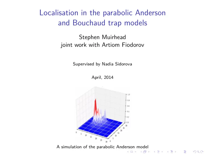
Localisation in the parabolic Anderson and Bouchaud trap models Stephen Muirhead joint work with Artiom Fiodorov Supervised by Nadia Sidorova April, 2014 A simulation of the parabolic Anderson model The parabolic Anderson model The parabolic
2 / 25
3 / 25
3 / 25
4 / 25
5 / 25
6 / 25
7 / 25
7 / 25
8 / 25
8 / 25
8 / 25
9 / 25
9 / 25
10 / 25
11 / 25
11 / 25
11 / 25
12 / 25
12 / 25
12 / 25
12 / 25
12 / 25
−|z−Z(1) t | γ
t
γ log log t 13 / 25
−|z−Z(1) t | γ
t
γ log log t
13 / 25
14 / 25
14 / 25
14 / 25
15 / 25
15 / 25
16 / 25
16 / 25
16 / 25
17 / 25
17 / 25
t
18 / 25
19 / 25
20 / 25
20 / 25
20 / 25
21 / 25
21 / 25
21 / 25
22 / 25
22 / 25
23 / 25
23 / 25
24 / 25
24 / 25
25 / 25