Linear Programming and Halfplane Intersection Carola Wenk 1 CMPS - - PowerPoint PPT Presentation

CMPS 3130/6130 Computational Geometry 1

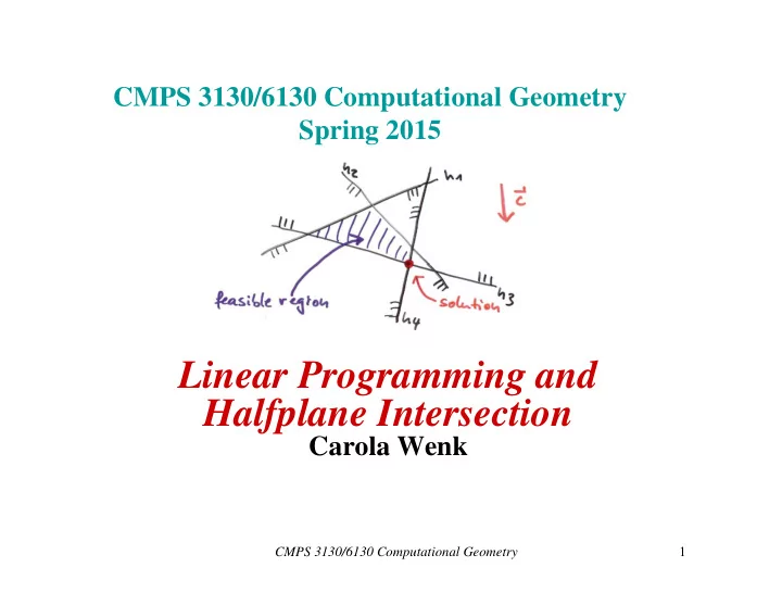
CMPS 3130/6130 Computational Geometry Spring 2015

Linear Programming and Halfplane Intersection

Carola Wenk

CMPS 3130/6130 Computational Geometry 2

Word Problem

A company produces tables and chairs. The profit for a chair is $2, and for a table $4. Machine group A needs 4 hours to produce a chair, and 6 hours to produce a table. Machine group B needs 2 hours to produce a chair, and 6 hours to produce a table. Per day there are at most 120 working hours for group A and at most 72 hours for group B. How can the company maximize profit? Variables: cA = # chairs produced on machine group A cB = # chairs produced on machine group B tA = # tables produced on machine group A tB = # tables produced on machine group B Constraints: 4cA +6tA ≤ 120 2cB +6tB ≤ 72 Objective function (profit): Maximize 2(cA+cB)+4(tA+tB)

CMPS 3130/6130 Computational Geometry 3

Linear Programming

Variables: x1,…,xd Constraints: h1: a11 x1+…+a1d xd ≤ b1 h2: a21 x1+…+a2d xd ≤ b2

. . .

hn: an1 x1+…+and xd ≤ bn Objective function: Maximize fc (x) = c1 x1+…+cd xd

• Each constraint hi is a half-space in Rd
• ⋂
• is the feasible region of the

linear program

• Maximizing fc (x) corresponds to

finding a point x that is extreme in direction c.

Linear program in d variables with n constraints

CMPS 3130/6130 Computational Geometry 4

Sub-Problem: Halfspace Intersection (in R2: Halfplane Intersection)

Given: A set H={h1, h2, …, hn} of halfplanes hi: ai x + bi y ≤ ci with constants ai, bi, ci ; for i=1,…,n . Find: ⋂

• , i.e., the feasible region of all points (x,y)R2

satisfying all n constraints at the same time. This is a convex polygonal region bounded by at most n edges.

intersection bounded intersection unbounded intersection empty intersection degenerated to a point

D&C Halfplane Intersection

Algorithm Intersect_Halfplanes(H): Input: A set H of n halfplanes in R2 Output: The convex polygonal region C= ⋂

• ∈

if |H|=1 then C = h , where H={h} else split H into two sets H1 and H2 of size n/2 each C1 = Intersect_Halfplanes(H1) C2 = Intersect_Halfplanes(H2) C = Intersect_Convex_Regions(C1, C2) return C

• Use a plane-sweep to develop an O(n)-time algorithm for

Intersect_Convex_Regions

• T(n) = 2T(n/2)+n

 T(n)O(n log n)

Incremental Linear Programming

• 2D linear program (LP)
• Assume the LP is bounded (otherwise add constraints)
• Assume there is one unique solution (if any);

take the lexicographically smallest solution

• Incremental approach: Add one halfplane after the other.

, … , ∩ ⋯ ∩ ⋂

• ∈

Let vi = unique optimal vertex for feasible region Ci , for 2 . Then ⊇ ⊇ … ⊇ , and hence if ∅ for some then

∅ for all .

Incremental Linear Programming

Lemma: Let 2≤i≤n. (i) If ∈ then (ii) If ∉ then ∅

• r ∈ the line bounding

Handling case (ii) involves solving a 1-dimensional LP on :

• The feasible region is just an interval,

that can be computed in linear time [rightmost left-bounded halfplane, leftmost right-bounded halfplane]

•  We can compute a new , or decide that the LP is

infeasible, in O(i) time

2D_Bounded_LP

Algorithm 2D_Bounded_LP(H , c ): Input: A two-dimensional LP (H , c ) Output: Report if (H , c ) is infeasible. Otherwise report the lexicographically smallest point that maximizes f c . Let , … , be the halfplanes of H Let be the corner of , which exists because LP is bounded for i=3 to n do if ∈ then else // Case (ii) point on that maximizes f c subject to constraints in if such a point does not exist then Report that the LP is infeasible break; return

• Runtime: ∑
• Storage:

Randomized Incremental LP

Depending on the insertion order of the halfplanes the runtime varies between O(n) and O(n2).  Randomize the input order of the halfplanes. Theorem: 2D_Randomized_Bounded_LP runs in O(n) expected time and O(n) deterministic space. Proof: Define a random variable 1, ∉ 0, The total time spent to resolve case (ii), over all , … , is

Randomized Incremental LP

We now need to bound the expected value E(∑ ∑

• and we know that ∉ .

Apply backwards analysis to bound :

– Fix , … , which determines . – Analyze what happened in last step when was added. – P(had to compute new optimal vertex when adding ) = P(optimal vertex changes when we remove a halfplane from )

• 
•  Total expected runtime is ∑
• 2 lines

defining vi