Likelihood Functions The likelihood function answers the question: - PowerPoint PPT Presentation

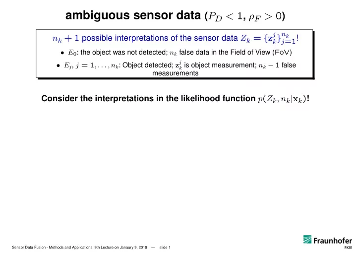
ambiguous sensor data ( P D < 1 , ρ F > 0 ) k } n k n k + 1 possible interpretations of the sensor data Z k = { z j j =1 ! • E 0 : the object was not detected; n k false data in the Field of View ( FoV ) • E j , j = 1 , . . . , n k : Object detected; z j k is object measurement; n k − 1 false measurements Consider the interpretations in the likelihood function p ( Z k , n k | x k ) ! Sensor Data Fusion - Methods and Applications, 9th Lecture on Janaury 9, 2019 — slide 1

ambiguous sensor data ( P D < 1 , ρ F > 0 ) k } n k n k + 1 possible interpretations of the sensor data Z k = { z j j =1 ! • E 0 : the object was not detected; n k false data in the Field of View ( FoV ) • E j , j = 1 , . . . , n k : Object detected; z j k is object measurement; n k − 1 false measurements Consider the interpretations in the likelihood function p ( Z k , n k | x k ) ! p ( Z k , n k | x k ) = p ( Z k , n k , ¬ D | x k ) + p ( Z k , n k , D | x k ) D = “object was detected” Sensor Data Fusion - Methods and Applications, 9th Lecture on Janaury 9, 2019 — slide 2

ambiguous sensor data ( P D < 1 , ρ F > 0 ) k } n k n k + 1 possible interpretations of the sensor data Z k = { z j j =1 ! • E 0 : the object was not detected; n k false data in the Field of View ( FoV ) • E j , j = 1 , . . . , n k : Object detected; z j k is object measurement; n k − 1 false measurements Consider the interpretations in the likelihood function p ( Z k , n k | x k ) ! p ( Z k , n k | x k ) = p ( Z k , n k , ¬ D | x k ) + p ( Z k , n k , D | x k ) D = “object was detected” = p ( Z k , n k |¬ D, x k ) P ( ¬ D | x k ) + p ( Z k , n k | D, x k ) P ( D | x k ) � �� � � �� � =1 − P D = P D detection probability P D sensor parameter: Sensor Data Fusion - Methods and Applications, 9th Lecture on Janaury 9, 2019 — slide 3

ambiguous sensor data ( P D < 1 , ρ F > 0 ) k } n k n k + 1 possible interpretations of the sensor data Z k = { z j j =1 ! • E 0 : the object was not detected; n k false data in the Field of View ( FoV ) • E j , j = 1 , . . . , n k : Object detected; z j k is object measurement; n k − 1 false measurements Consider the interpretations in the likelihood function p ( Z k , n k | x k ) ! p ( Z k , n k | x k ) = p ( Z k , n k , ¬ D | x k ) + p ( Z k , n k , D | x k ) D = “object was detected” = p ( Z k , n k |¬ D, x k ) P ( ¬ D | x k ) + p ( Z k , n k | D, x k ) p ( D | x k ) n k � = p ( Z k | n k , ¬ D, x k ) p ( n k |¬ D, x k ) (1 − P D ) + P D p ( Z k , n k , j | D, x k ) � �� � � �� � j =1 = | FoV | − nk = p F ( n k ) Poisson distributed in #, uniformly distributed in the FoV false measurements: Sensor Data Fusion - Methods and Applications, 9th Lecture on Janaury 9, 2019 — slide 4

ambiguous sensor data ( P D < 1 , ρ F > 0 ) k } n k n k + 1 possible interpretations of the sensor data Z k = { z j j =1 ! • E 0 : the object was not detected; n k false data in the Field of View ( FoV ) • E j , j = 1 , . . . , n k : Object detected; z j k is object measurement; n k − 1 false measurements Consider the interpretations in the likelihood function p ( Z k , n k | x k ) ! p ( Z k , n k | x k ) = p ( Z k , n k , ¬ D | x k ) + p ( Z k , n k , D | x k ) D = “object was detected” = p ( Z k , n k |¬ D, x k ) P ( ¬ D | x k ) + p ( Z k , n k | D, x k ) p ( D | x k ) n k � = p ( Z k | n k , ¬ D, x k ) p ( n k |¬ D, x k ) (1 − P D ) + P D p ( Z k , n k , j | D, x k ) j =1 n k � = | FoV | − n k p F ( n k ) (1 − P D ) + P D p ( Z k | n k , j, D, x k ) p ( j | n k , D ) p ( n k | D ) � �� � � �� � � �� � j =1 | FoV | − ( nk − 1) N ( z j =1 /n k = p F ( n k − 1) k ; Hx k , R ) p F ( n k ) = ( ρ F | FoV | ) − nk e − ρ F | FoV | Insert Poisson distribution: n k ! Sensor Data Fusion - Methods and Applications, 9th Lecture on Janaury 9, 2019 — slide 5

ambiguous sensor data ( P D < 1 , ρ F > 0 ) k } n k n k + 1 possible interpretations of the sensor data Z k = { z j j =1 ! • E 0 : the object was not detected; n k false data in the Field of View ( FoV ) • E j , j = 1 , . . . , n k : Object detected; z j k is object measurement; n k − 1 false measurements Consider the interpretations in the likelihood function p ( Z k , n k | x k ) ! p ( Z k , n k | x k ) = p ( Z k , n k , ¬ D | x k ) + p ( Z k , n k , D | x k ) D = “object was detected” = p ( Z k , n k |¬ D, x k ) P ( ¬ D | x k ) + p ( Z k , n k | D, x k ) p ( D | x k ) n k � = p ( Z k | n k , ¬ D, x k ) p ( n k |¬ D, x k ) (1 − P D ) + P D p ( Z k , n k , j | D, x k ) j =1 n k � = | FoV | − n k p F ( n k ) (1 − P D ) + P D p ( Z k | n k , j, D, x k ) p ( j | n k , D ) p ( n k | D ) j =1 n k � �� � � z j = e − ρF | FoV | ρ n k − 1 (1 − P D ) ρ F + P D N k ; Hx k , R F n k ! j =1 Sensor Data Fusion - Methods and Applications, 9th Lecture on Janaury 9, 2019 — slide 6

Likelihood Functions The likelihood function answers the question: What does the sensor tell about the state x of the object? (input: sensor data, sensor model) • ideal conditions, one object: P D = 1 , ρ F = 0 p ( z k | x k ) = N ( z k ; Hx k , R ) at each time one measurement: • real conditions, one object: P D < 1 , ρ F > 0 k , . . . , z n k at each time n k measurements Z k = { z 1 k } ! n k � N � z j k ; Hx k , R � p ( Z k , n k | x k ) ∝ (1 − P D ) ρ F + P D j =1 7 Introduction to Sensor Data Fusion: Methods and Applications — 9th Lecture on January 9, 2019 slide 7

Bayes Filtering for: P D < 1 , ρ F > 0 , well-separated objects accumulated data Z k = { Z k , Z k − 1 } current data Z k = { z j k } m k state x k , j =1 , interpretation hypotheses E k for Z k � object not detected, 1 − P D m k + 1 interpretations z k ∈ Z k from object, P D • tree structure: H k = ( E H k , H k − 1 ) ∈ H k interpretation histories H k for Z k • current: E H k , pre histories: H k − i � � � x k | Z k � � x k , H k | Z k � � H k | Z k � p � x k | H k , Z k � p = p = p ‘mixture’ density � �� � � �� � H k H k weight! given H k : unique 8 Introduction to Sensor Data Fusion: Methods and Applications — 9th Lecture on January 9, 2019 slide 8

Closer look: P D < 1 , ρ F > 0 , well-separated targets � � � p ( x k − 1 |Z k − 1 ) = p H k − 1 N x k − 1 ; x H k − 1 , P H k − 1 filtering (at time t k − 1 ): H k − 1 prediction (for time t k ): � p ( x k |Z k − 1 ) d x k − 1 p ( x k | x k − 1 ) p ( x k − 1 |Z k − 1 ) = (M ARKOV model) � � x k ; Fx H k − 1 , FP H k − 1 F ⊤ + D � = p H k − 1 N (IMM also possible) H k − 1 measurement likelihood: m k � p ( Z k | E j k , x k , m k ) P ( E j ( E j p ( Z k , m k | x k ) = k | x k , m k ) k : interpretations) j =0 m k � � � z j ∝ (1 − P D ) ρ F + P D N k ; Hx k , R ( H , R , P D , ρ F ) j =1 filtering (at time t k ): p ( x k |Z k ) p ( Z k , m k | x k ) p ( x k |Z k − 1 ) ∝ (B AYES ’ rule) � � � = p H k N x k ; x H k , P H k (Exploit product formula) H k Sensor Data Fusion - Methods and Applications, 9th Lecture on Janaury 9, 2019 — slide 9

Problem: Growing Memory Disaster: m data, N hypotheses → N m +1 continuations radical solution: mono-hypothesis approximation Sensor Data Fusion - Methods and Applications, 9th Lecture on Janaury 9, 2019 — slide 10

Problem: Growing Memory Disaster: m data, N hypotheses → N m +1 continuations radical solution: mono-hypothesis approximation • gating: Exclude competing data with || ν i k | k − 1 || > λ ! → K ALMAN filter (KF) + very simple, − λ too small: loss of target measurement Sensor Data Fusion - Methods and Applications, 9th Lecture on Janaury 9, 2019 — slide 11

Problem: Growing Memory Disaster: m data, N hypotheses → N m +1 continuations radical solution: mono-hypothesis approximation • gating: Exclude competing data with || ν i k | k − 1 || > λ ! → K ALMAN filter (KF) + very simple, − λ too small: loss of target measurement • Force a unique interpretation in case of a conflict! look for smallest statistical distance: min i || ν i k | k − 1 || → Nearest-Neighbor filter (NN) Sensor Data Fusion - Methods and Applications, 9th Lecture on Janaury 9, 2019 — slide 12

Problem: Growing Memory Disaster: m data, N hypotheses → N m +1 continuations radical solution: mono-hypothesis approximation • gating: Exclude competing data with || ν i k | k − 1 || > λ ! → K ALMAN filter (KF) + very simple, − λ too small: loss of target measurement • Force a unique interpretation in case of a conflict! look for smallest statistical distance: min i || ν i k | k − 1 || Nearest-Neighbor filter (NN) → + one hypothesis, − hard decision, − not adaptive • global combining: Merge all hypotheses! → PDAF, JPDAF filter + all data, + adaptive, − reduced applicability Sensor Data Fusion - Methods and Applications, 9th Lecture on Janaury 9, 2019 — slide 13

Sensor Data Fusion - Methods and Applications, 9th Lecture on Janaury 9, 2019 — slide 14

Sensor Data Fusion - Methods and Applications, 9th Lecture on Janaury 9, 2019 — slide 15

Sensor Data Fusion - Methods and Applications, 9th Lecture on Janaury 9, 2019 — slide 16

Sensor Data Fusion - Methods and Applications, 9th Lecture on Janaury 9, 2019 — slide 17

Sensor Data Fusion - Methods and Applications, 9th Lecture on Janaury 9, 2019 — slide 18