Lessons learned from the theory and practice of Simulated data - One - PowerPoint PPT Presentation

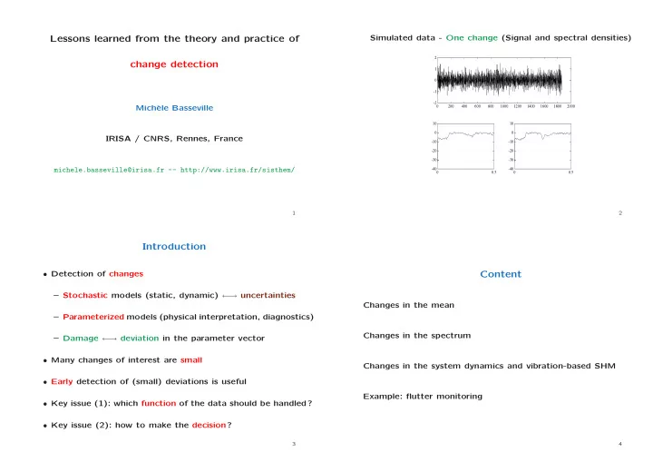
Lessons learned from the theory and practice of Simulated data - One change (Signal and spectral densities) 2 change detection 1 0 -1 -2 0 200 400 600 800 1000 1200 1400 1600 1800 2000 Mich` ele Basseville 10 10 0 0 IRISA / CNRS, Rennes, France -10 -10 -20 -20 -30 -30 -40 -40 michele.basseville@irisa.fr -- http://www.irisa.fr/sisthem/ 0 0.5 0 0.5 1 2 Introduction • Detection of changes Content – Stochastic models (static, dynamic) ← → uncertainties Changes in the mean – Parameterized models (physical interpretation, diagnostics) Changes in the spectrum – Damage ← → deviation in the parameter vector • Many changes of interest are small Changes in the system dynamics and vibration-based SHM • Early detection of (small) deviations is useful Example: flutter monitoring • Key issue (1): which function of the data should be handled? • Key issue (2): how to make the decision? 3 4

Changes in the mean Hypothesis testing Hypotheses H 0 H 1 Key concepts - Independent data Simple θ 0 θ 1 Known parameter values Likelihood p θ ( y i ) Composite Θ 0 Θ 1 Unknown parameter values ln p θ 1 ( y i ) ∆ Simple hypotheses : Likelihood ratio test Log-likelihood ratio s i = p θ 0 ( y i ) If Λ N ≥ λ / S N ≥ h : decide H 1 , H 0 otherwise E θ 0 ( s i ) < 0 E θ 1 ( s i ) > 0 Composite hypotheses : Generalized likelihood ratio (GLR) p θ 1 ( Y N � 1 ) i p θ 1 ( y i ) θ 1 ( Y N = sup θ 1 ∈ Θ 1 p θ 1 ( Y N p � 1 ) ∆ 1 ) Likelihood ratio Λ N = 1 ) = � Λ N 1 ) = p θ 0 ( Y N � i p θ 0 ( y i ) sup θ 0 ∈ Θ 0 p θ 0 ( Y N θ 0 ( Y N p � 1 ) ∆ � N Log-likelihood ratio S N = ln Λ N = i =1 s i Maximize the likelihoods w.r.t. unknown values of θ 0 and θ 1 5 6 On-line change detection, unknown onset time Simple case: Known θ 1 - CUSUM algorithm θ o θ 1 t Ratio of likelihoods under H 0 and H 1 : o � t 0 − 1 n � k � k 1 ? p θ 0 ( y i ) · i = t 0 p θ 1 ( y i ) i = t 0 p θ 1 ( y i ) i =1 = Λ k = t 0 � k � k i =1 p θ 0 ( y i ) i = t 0 p θ 0 ( y i ) Hypothesis H 0 θ = θ 0 (1 ≤ i ≤ k ) known Maximize over the unknown onset time t 0 : j − 1 k ∆  � � � i =1 p θ 0 ( y i ) · ( t 0 ) k = arg max i = j p θ 1 ( y i )  θ 0 (1 ≤ i < t 0 )    1 ≤ j ≤ k    Hypothesis H 1 ∃ t 0 s.t. θ =     θ 1 ( t 0 ≤ i ≤ k )  Λ k   = arg max j 1 ≤ j ≤ k S k S k j = ln Λ k = arg max j , j 1 ≤ j ≤ k t a = min { k ≥ 1 : g k ≥ h } decision function Alarm time t a : ∆ 1 ≤ j ≤ k S k = ln Λ k g k = max � Estimated onset time: t 0 j ˆ t 0 7 8

CUSUM algorithm (Contd.) Lesson 1 CUSUM algorithm (Contd.) - Gaussian example    − ( y i − µ ) 2 1 ∆ 1 ≤ j ≤ k S k g k = max θ ∆ p θ ( y ) ∆ N ( µ, σ 2 ) ,   √   = µ, = 2 π exp j   2 σ 2  σ 1 ≤ j ≤ k S j 1 ≤ j ≤ k S j S k 1 = S k ∆ = 1 − min 1 − m k , m k = min 1 ln p µ 1 ( y i ) s i = p µ 0 ( y i ) min { k ≥ 1 : S k 1 ≥ m k + h } t a = Adaptative threshold 1 � � ( y i − µ 0 ) 2 − ( y i − µ 1 ) 2 = 2 σ 2 ( g k − 1 + s k ) + g k =   ν  y i − µ 0 − ν  , ν = µ 1 − µ 0 =   σ 2 2 � � + , ∆ S k = N k − 1 · I ( g k − 1 ) + 1 g k = N k k − N k +1 k S k � involves i =1 y i : Integrator (with adaptive threshold) � t a − N t a + 1 1 ( t 0 ) k = Sliding window with adaptive size 9 10 Composite case: Unknown θ 1 CUSUM algorithm - Gaussian example (Contd.) 7 6 Modified CUSUM algorithms 5 4 3 2 1 Minimum magnitude of change 0 -1 -2 -3 0 5 10 15 20 25 30 35 40 45 50 y k Weighted CUSUM 10 0 -10 -20 GLR algorithm -30 -40 -50 S k 0 5 10 15 20 25 30 35 40 45 50 Double maximization 1 90 80 70 60 50 S k g k = max sup j ( θ 1 ) 40 1 ≤ j ≤ k 30 θ 1 20 10 0 0 5 10 15 20 25 30 35 40 45 50 g k Gaussian case, additive faults: second maximization explicit. 11 12

Changes in the spectrum Unknown θ 1 - Gaussian example (Contd.) Key concepts - Dependent data Minimum magnitude of change ν m Lesson 2 Conditional likelihood p θ ( y i |Y i − 1 ) 1 Decreasing mean Increasing mean ln p θ 1 ( y i |Y i − 1 ) ∆ 1 Log-likelihood ratio s i = p θ 0 ( y i |Y i − 1 ) 1      y i − µ 0 + ν m  y i − µ 0 − ν m ∆ ∆ T k � k U k � k =   =     1 i =1 1 i =1 2 2 E θ 0 ( s i ) < 0 E θ 1 ( s i ) > 0 ∆ = max 1 ≤ j ≤ k T j = min 1 ≤ j ≤ k U j ∆ M k m k 1 1 i p θ 1 ( y i |Y i − 1 p θ 1 ( Y N � 1 ) ) ∆ 1 Likelihood ratio Λ N = = i p θ 0 ( y i |Y i − 1 p θ 0 ( Y N � 1 ) ) t a = min { k ≥ 1 : M k − T k t a = min { k ≥ 1 : U k 1 1 ≥ h } 1 − m k ≥ h } ∆ � N Log-likelihood ratio S N = ln Λ N = i =1 s i 13 14 Key concepts - Dependent data (Contd.) Key concepts - Dependent data (Contd.) θ 0 : reference parameter, known (or identified) Which residuals? Lesson 3 Y k : N -size sample of new measurements • Likelihood ratio computationally complex Build a residual ζ significantly non zero when damage • Efficient score : likelihood sensitivity w.r.t. parameter vector Residual ↔ Estimating function ζ N ( θ, Y N 1 ) • Other estimating fonctions Characterized by : E θ 0 ζ N ( θ, Y N ⇐ ⇒ 1 ) = 0 θ = θ 0 Innovation not sufficient for monitoring the dynamics. Mean sensitivity J ( θ 0 ) and covariance Σ( θ 0 ) of ζ N ( θ 0 ) 15 16

Key concepts - Dependent data (Contd.) Changes in the dynamics and vibration-based SHM The residual is asymptotically Gaussian Structural monitoring : Eigenstructure monitoring  N (  0 , Σ( θ 0 )) if P θ 0         ζ N ( θ 0 ) →   N ( J ( θ 0 ) δθ, Σ( θ 0 ))  if P θ 0 + δθ small deviations     √   N  X k +1 = F X k + V k F Φ λ = λ Φ λ           (On-board) χ 2 -test in the residual     ∆    Y k = H X k ϕ λ = H Φ λ    N Σ − 1 J ( J T Σ − 1 J ) − 1 J T Σ − 1 ζ N ζ T ≥ h   Λ modes θ ∆   Canonical parameter : =      vec Φ  mode shapes Noises and uncertainty on θ 0 taken into account. 17 18 Example: flutter monitoring Detecting structural changes Monitoring a damping coefficient • Reference data → covariances → Hankel matrix H 0 • Test ρ ≥ ρ c against ρ < ρ c Left null space S s.t. S T H 0 = 0 ( S T O ( θ 0 ) = 0 ) • Write the subspace-based residual ζ • Fresh data → covariances → Hankel matrix H 1 as a cumulative sum = S T H 1 � = 0 Check if ζ ∆ • Introduce a minimum change magnitude (actual change magnitude unknown) ζ asympt. Gaussian, test: χ 2 in ζ • Run two CUSUM tests in parallel (actual change direction unknown) 19 20

Flutter monitoring (Contd) Application to real datasets Ariane booster launcher during a launch scenario on the ground (not during a real flight test) Running the test with 2 critical values With Laurent M´ evel, Maurice Goursat, Albert Benveniste Free COSMAD Toolbox to used with Scilab http://www.irisa.fr/sisthem/cosmad/ Automatic identification. Each symbol: processing 5 sec. data. 21 22 Conclusion Advanced statistical signal processing mandatory for SHM A statistical framework enlightens the meaning and On-line test for ρ c = ρ 0 = ρ (1) . c increases the power of a number of familiar operations integration, averaging, sensitivity, adaptive thresholds & windows Change detection useful for (vibration-based) SHM Current investigations On-line test for ρ c = ρ 0 = ρ (2) < ρ (1) . c c • flutter monitoring (with Dassault, Airbus), Bottom: − g − n reflects ρ < ρ c . Top: g + • handling the temperature effect on civil structures (with LCPC) n reflects ρ > ρ c . 23 24