Lecture 13 - BRDFs Welcome! , = (, ) , - PowerPoint PPT Presentation
INFOMAGR Advanced Graphics Jacco Bikker - November 2017 - February 2018 Lecture 13 - BRDFs Welcome! , = (, ) , + , , ,
INFOMAGR – Advanced Graphics Jacco Bikker - November 2017 - February 2018 Lecture 13 - “BRDFs” Welcome! 𝑱 𝒚, 𝒚 ′ = 𝒉(𝒚, 𝒚 ′ ) 𝝑 𝒚, 𝒚 ′ + න 𝝇 𝒚, 𝒚 ′ , 𝒚 ′′ 𝑱 𝒚 ′ , 𝒚 ′′ 𝒆𝒚′′ 𝑻
Today’s Agenda: Exam Questions: Sampler (3) Phong BRDF Microfacets Demo Time Quo Vadis
Advanced Graphics – BRDFs 3 Exam Questions In path tracing, we can reduce variance by using cosine weighted sampling of the hemisphere, rather than uniform sampling, for diffuse surfaces. a) Why does this reduce variance? b) When using cosine weighted sampling, the result remains unbiased. What does unbiased mean?
Advanced Graphics – BRDFs 4 Exam Questions An exam can be seen as a Monte-Carlo process. Expain why.
Advanced Graphics – BRDFs 5 Exam Questions After reading the probability tutorial, answer these: a) What is a definite integral? b) What do we mean by an analytical solution? c) How is the Riemann sum defined (mathematically)? d) What is ‘ univariate ’? e) What is ‘aliasing’? f) Define, in your own words, ‘expected value’. g) What is ‘deviation’ in the context of probability theory? And, finally: When using importance sampling, we assume that for 𝑂 = ∞ , 𝑐 𝑞 𝑦 𝑒𝑦 = 1 . Provide one 𝑐−𝑏 𝑔(𝑌) 𝑐−𝑏 𝑂 𝑂 𝑂 σ 𝑗=1 𝑂 σ 𝑗=1 𝑞(𝑌) = 𝑔(𝑌) , if 𝑏 example for which this is not true.
Today’s Agenda: Exam Questions: Sampler (3) Phong BRDF Microfacets Demo Time Quo Vadis
Advanced Graphics – BRDFs 7 Phong BRDFs, Recap Recall that a BRDF defines the relation between incoming and outgoing radiance for directions and a surface point: 𝑠 𝑦, 𝜄 𝑗 , 𝜄 𝑝 = 𝑀 𝑝 (𝑦, 𝜄 𝑝 ) 𝑀 𝑝 (𝑦, 𝜄 𝑝 ) What about materials that are 𝑔 𝐹 𝑗 (𝑦, 𝜄 𝑗 ) = 𝑀 𝑗 𝑦, 𝜄 𝑗 cos 𝜄 𝑗 not purely specular, nor diffuse? 𝑜 𝑜 𝑜 𝜄 𝑗 𝜄 𝑝 𝑦
Advanced Graphics – BRDFs 8 Phong BRDFs, Recap We already know how to do materials that are diffuse and shiny. But that gets us good looking marble floors, not glossy reflections. 50% diffuse, 50% specular, 50% diffuse, 50% glossy (or: 100% glossy)
Advanced Graphics – BRDFs 9 Phong Glossy Reflection Glossy reflections: sending out rays in random directions close to the reflected vector. Simple solution: 𝑆 = 𝑠𝑓𝑔𝑚𝑓𝑑𝑢(𝑊, 𝑂); 𝑄 = 𝐽 + 𝑆 + 𝑡𝑑𝑏𝑚𝑓(𝑠𝑏𝑜𝑒𝑝𝑛𝑄𝑝𝑗𝑜𝑢𝐽𝑜𝑇𝑞ℎ𝑓𝑠𝑓(), 𝑡𝑞𝑓𝑑𝑣𝑚𝑏𝑠𝑗𝑢𝑧) 𝑆 = 𝑜𝑝𝑠𝑛𝑏𝑚𝑗𝑨𝑓(𝑄 − 𝐽); 𝑶 Or: 𝑆 = 𝑠𝑓𝑔𝑚𝑓𝑑𝑢(𝑊, 𝑂); 𝑄 = 𝐽 + 𝑆 + 𝑡𝑑𝑏𝑚𝑓(𝑠𝑏𝑜𝑒𝑝𝑛𝐸𝑗𝑠𝑓𝑑𝑢𝑗𝑝𝑜𝐽𝑜𝐼𝑓𝑛𝑗𝑡𝑞ℎ𝑓𝑠𝑓𝐷𝑝𝑡𝑗𝑜𝑓𝑋𝑓𝑗ℎ𝑢𝑓𝑒(𝑆), 𝑡𝑞𝑓𝑑𝑣𝑚𝑏𝑠𝑗𝑢𝑧) 𝑆 = 𝑜𝑝𝑠𝑛𝑏𝑚𝑗𝑨𝑓(𝑄 − 𝐽);
Advanced Graphics – BRDFs 10 Phong 𝑑𝑝𝑡 𝑓𝑦𝑞 𝜄 =? න 𝛻 Glossy Reflection න cos 𝜄 = 𝜌 𝛻 In OpenGL, shading is defined as follows*: 𝑓𝑦𝑞𝑝𝑜𝑓𝑜𝑢 𝐽 𝑦 = 𝑙 𝑏𝑛𝑐𝑗𝑓𝑜𝑢 𝐽 𝑏𝑛𝑐𝑗𝑓𝑜𝑢 + 𝑙 𝑒𝑗𝑔𝑔𝑣𝑡𝑓 𝑂 ∙ 𝑀 𝑛 + 𝑙 𝑡𝑞𝑓𝑑𝑣𝑚𝑏𝑠 𝑆 𝑛 ∙ 𝑊 𝐽 𝑛 𝑛∈𝑚𝑗ℎ𝑢𝑡 𝑆 𝑛 where 𝑀 𝑛 𝑙 𝑏𝑛𝑐𝑗𝑓𝑜𝑢 , 𝑙 𝑒𝑗𝑔𝑔𝑣𝑡𝑓 𝑏𝑜𝑒 𝑙 𝑡𝑞𝑓𝑑𝑣𝑚𝑏𝑠 are material properties (typically: rgb); 𝑆 𝑛 is the vector 𝑀 𝑛 reflected in the 𝑊 normal 𝑂 ; 𝑂 𝐽 𝑛 is the illumination from light 𝑛 . 𝑦 *: Bui-Tuong Phong, Illumination for Computer Generated Images, 1975.
Advanced Graphics – BRDFs 11 Phong Blinn-Phong BRDF (images: Disney BRDF Explorer )
Advanced Graphics – BRDFs 12 Phong Modified Phong BRDF
Advanced Graphics – BRDFs 13 Phong Fixing Phong Recall the requirements for a proper BRDF: Should be positive: 𝑔 𝑠 𝜕 𝑝 , 𝜕 𝑗 ≥ 0 Helmholtz reciprocity should be obeyed: 𝑔 𝑠 𝜕 𝑝 , 𝜕 𝑗 = 𝑔 𝑠 𝜕 𝑗 , 𝜕 𝑝 Energy should be conserved: 𝛻 𝑔 𝑠 𝜕 𝑝 , 𝜕 𝑗 cos 𝜄 𝑝 𝑒𝜕 𝑝 ≤ 1 BRDFs obeying these rules are called physically plausible. For a path tracer, we have additional requirements: 1. It ‘would be nice’ if we could generate a random direction proportional to the BRDF (IS) 2. We need to be able to calculate the probability density (importance) for a given direction (for MIS).
Advanced Graphics – BRDFs 14 Phong 𝑨 Fixing Phong 1. Sampling the specular lobe proportional to the BRDF: 𝑦 𝑆 ∙ 𝑊 1 𝑆 ∙ 𝑊 2 𝑆 ∙ 𝑊 10 𝑆 ∙ 𝑊 50 𝑧 Sampling proportional to Sampling proportional to 𝑆 ∙ 𝑊 𝛽 , according to the G.I.C. : 𝑂 ∙ 𝑀 , according to the G.I.C. : 2 𝛽+1 , 𝑦 = cos 2𝜌𝑠 𝑦 = cos 2𝜌𝑠 1 − 𝑠 2 𝑢 = 𝑠 1 − 𝑢 1 1 2 𝑧 = sin 2𝜌𝑠 1 − 𝑢 𝑧 = sin 2𝜌𝑠 1 − 𝑠 2 1 1 𝑨 = 𝑢 𝑨 = 𝑠 2
Advanced Graphics – BRDFs 15 Phong 𝑶 𝑨 Tangent / Local Space Setting up a local coordinate system in 2D: First axis is the normal; Second axis is perpendicular to normal. Good choice for 𝑋 : 𝑼 𝑂 = 𝑜 𝑦 𝑋 = (0,1,0) if abs( 𝑜 𝑦 ) > 0.99; 𝑈 = −𝑜. 𝑧 𝑋 = 1,0,0 otherwise. 𝑜. 𝑦 Setting up a local coordinate system in 3D: 𝑧 𝑪 𝑂 = 𝑜 𝑈 = 𝑜𝑝𝑠𝑛𝑏𝑚𝑗𝑨𝑓(𝑂 × 𝑋) 𝐶 = 𝑈 × 𝑂 where 𝑋 is a random unit vector; 𝑋 ≠ 𝑂 .
Advanced Graphics – BRDFs 16 Phong 𝑶 Tangent / Local Space Converting a vector from world space to local space: 𝑄 𝑄 ∙ 𝑈 𝑦 𝑄 = 𝑄 ∙ 𝐶 𝑧 𝑄 𝑄 ∙ 𝑂 𝑨 𝑼 Local space to world space: 𝑄 𝑥𝑝𝑠𝑚𝑒 = 𝑁 × 𝑄 𝑚𝑝𝑑𝑏𝑚 𝑪 = 𝑄 𝑦 𝑈 + 𝑄 𝑧 𝐶 + 𝑄 𝑨 𝑂
Advanced Graphics – BRDFs 17 Phong Normalizing the Lobe A material cannot reflect more energy than it receives: We thus scale the BRDF by the inverse of its integral over the hemisphere. 1 For the Lambertian BRDF: 𝑡𝑑𝑏𝑚𝑓 = 𝜌 (because cos 𝜄 integrates to 𝜌 ) 𝛽+1 For the cosine lobe, the scale is 2𝜌 (*). However, there is a problem: 𝑜 𝑜 𝑜 *: Physically Based Rendering, page 969; also see: http://www.farbrausch.de/~fg/stuff/phong.pdf
Advanced Graphics – BRDFs 18 1 𝛽+2 2𝜌 𝑑𝑝𝑡 𝛽 𝜒 : 𝑔 𝑠 𝑦, 𝜄 𝑗 , 𝜄 𝑝 = 𝑙 𝑒 𝜌 + 𝑙 𝑡 Phong Total hemispherical reflection (note: integrating over outgoing directions, since these cannot exceed 1): 𝜍 𝑦, 𝜄 𝑝 = න 𝑔 𝑠 𝑦, 𝜄 𝑗 , 𝜄 𝑝 cos θ 𝑝 𝑒𝜕 𝑝 The Modified Phong BRDF Ω 1 𝛽 + 2 2𝜌 𝑑𝑝𝑡 𝛽 𝜒) cos θ 𝑝 𝑒𝜕 𝑝 = න (𝑙 𝑒 𝜌 + 𝑙 𝑡 The Phong BRDF has problems: Ω 𝛽 + 2 𝑑𝑝𝑡 𝛽 𝜒 cos θ 𝑝 𝑒𝜕 𝑝 = 𝑙 𝑒 + 𝑙 𝑡 2𝜌 න 1. it does not doesn’t obey the Helmholtz reciprocity rule . Ω The last integral is maximal when the incoming light 2. We can only estimate the integral of the lobe, since it arrives along the normal; in this case 𝜒 = 𝜄 𝑝 , and the intersects the surface. integral is 2𝜌 / (𝑜 + 2) . Therefore, in this case: 𝜍 𝑦, 𝜄 𝑝 = 𝑙 𝑒 + 𝑙 𝑡 Compensating for the intersection: Modified Phong BRDF. and conservation of energy is guaranteed iff: 1 𝛽 + 2 2𝜌 𝑑𝑝𝑡 𝛽 𝜒 𝑔 𝑠 𝑦, 𝜄 𝑗 , 𝜄 𝑝 = 𝑙 𝑒 𝜌 + 𝑙 𝑡 𝑙 𝑒 + 𝑙 𝑡 ≤ 1. where 𝜒 is the angle between the view vector and the reflected light vector. For 𝑙 𝑒 + 𝑙 𝑡 < 1 , this guarantees energy preservation*. *: Lafortune & Willems, Using the Modified Phong Reflectance Model for Physically Based Rendering, 1994.
Advanced Graphics – BRDFs 19 Phong The Modified Phong BRDF Despite the kludges, we now have a decent BRDF for glossy materials. We can sample it: 2 𝛽+1 , 𝑦 = cos 2𝜌𝑠 𝑢 = 𝑠 1 − 𝑢 1 2 𝑧 = sin 2𝜌𝑠 1 − 𝑢 1 𝑨 = 𝑢 Normalize it: And finally, we can blend it with the Lambertian BRDF: 𝛽 + 2 2𝜌 𝑑𝑝𝑡 𝛽 𝜒 Define a probability 𝑞 of sampling Phong; Draw a random number 𝑠 0 ; Sample Phong if 𝑠 0 < 𝑞 , Lambert otherwise; 𝛽 + 2 2𝜌 𝑑𝑝𝑡 𝛽 𝜒 We have a PDF: Combine PDFs: 𝑄𝐸𝐺 = 𝑞 𝑄𝐸𝐺 𝑞ℎ𝑝𝑜 + 1 − 𝑞 𝑄𝐸𝐺 𝑒𝑗𝑔𝑔
Today’s Agenda: Exam Questions: Sampler (3) Phong BRDF Microfacets Demo Time Quo Vadis
Advanced Graphics – BRDFs 21 Microfacet BRDFs Without Issues We now have two BRDFs without problems: 1. The Lambertian BRDF 2. The pure specular BRDF These are plausible and can be sampled. The PDF is also clear. And, we have the somewhat kludged modified Phong BRDF.
Recommend
More recommend
Explore More Topics
Stay informed with curated content and fresh updates.
