Lagrangian/Eulerian Multiphysics Modeling and DeRham Complex Based - - PowerPoint PPT Presentation

Photos placed in horizontal position with even amount of white space between photos and header

Sandia National Laboratories is a multi-program laboratory managed and operated by Sandia Corporation, a wholly owned subsidiary of Lockheed Martin Corporation, for the U.S. Department of Energy’s National Nuclear Security Administration under contract DE-AC04-94AL85000. SAND NO. 2013-XXXXP

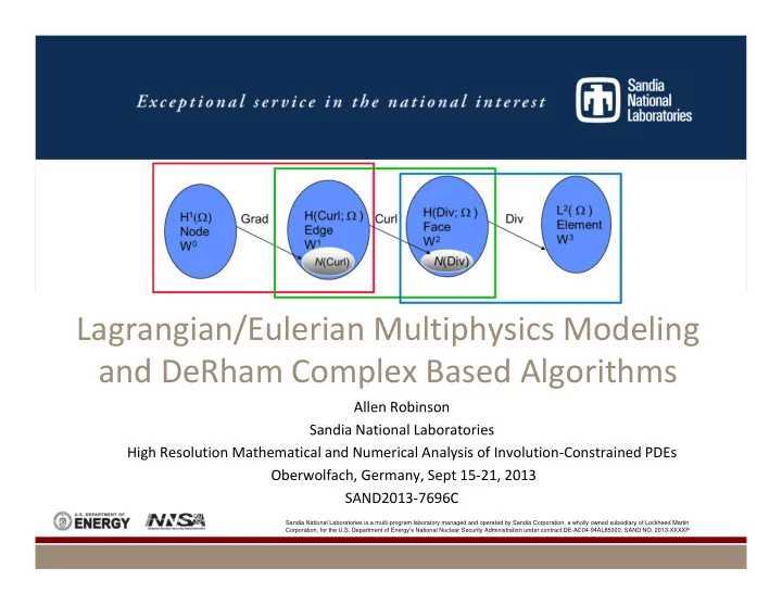
Lagrangian/Eulerian Multiphysics Modeling and DeRham Complex Based Algorithms

Allen Robinson Sandia National Laboratories High Resolution Mathematical and Numerical Analysis of Involution‐Constrained PDEs Oberwolfach, Germany, Sept 15‐21, 2013 SAND2013‐7696C

Outline

• Lagrangian/Eulerian Numerical Methods
• DeRham Tour
• Inverse Deformation Gradient
• Magnetic Flux Density
• Volume Remapping
• A possible cross‐cutting algorithm
• Conclusion

2

3

• Lagrangian:
• Mesh moves with material points.
• Mesh-quality may deteriorate over time
• REMESH
• Mesh-quality is adjusted to improve solution-

quality or robustness.

• Eulerian sets new mesh to original location
• REMAP
• Algorithm transfers dependent variables to the

new mesh.

Arbitrary Lagrangian/Eulerian (ALE)

4

• Lagrangian:
• The kinematic complexity is simplified due to

embedding in the Lagrangian frame.

• Use of mimetic operators keeps the solution in the

right space.

• Remesh:
• Nothing special
• Remap:
• Algorithm looks like a “constrained transport”

algorithm in some way.

• The algorithm of necessity is un-split.

What happens with Involution Constraints and ALE?

Geometric Structure and Numerical Methods

• The structure of the equations is related to their geometric origins.
• This geometry can reappear in effective numerical methods.
• The deRham structure shown below is used to discuss issues of “compatible

discretizations.”

• These are related to 0‐forms, 1‐forms, 2‐forms and 3‐forms.
• Transport theorems are associated with the kinematics of such mathematical ideas.
• Presentation is “color coded”

H1) Node W0 H(Curl;  ) Edge W1 H(Div;  ) Face W2 L2(  ) Element W3

N(Curl)

N(Div) Grad Curl Div

Circulation Transport Theorem

d dt A

1 dx A2 dy A 3 dz t (U )



 d dt Ak dxk

t (U )



  Ak dxk 

t (U )



Ak vk xl dxl   Ak dxk 

t (U )



A

l

vl xk dxk  (Ak t  vl Ak xl 

t (U )



A

l

vl xk )dxk  (At  (Av)  v ( A))dx

t (U )



Surface Flux Transport Theorem

d dt B

1 dy dz B2 dzdx B3 dxdy t (U )



 d dt Bk dak

t (U )



  B

1 dy dz  B 1(v

x

t (U )



dx  v y dy  v z dz)dz B

1dy(w

x dx  w y dy  w z dz)...  (  Bi 

t (U )



Bi vk xk  Bk vi xk )dai  (Bt  (B v) vdivB)i

t (U )



dai

Volume Transport

d dt  dv

t (U )



 d dt ((X ,t),t)J(X ,t)dV

U



   ((X ,t),t)J (X ,t) ((X ,t),t)  J (X ,t)dV

U



 (t  v)J (X ,t) ((X ,t)(div v)J (X ,t)dV

U



 (     div v)dv

t (U )



 (t  div (v))dv

t (U )



 (t  div (v))dv

t (U )



Solid Kinematics

H1) Node W0 H(Curl;  ) Edge W1 H(Div;  ) Face W2 L2(  ) Element W3

N(Curl)

N(Div) Grad Curl Div

Solid Kinematics

x(a,t)

(Current) Spatial Coordinates

. x(a,t) . a

(Reference) Material Coordinates

Deformation gradient and inverse: Symmetric Positive Definite (Stretch) Tensor Proper Orthogonal (Rotation) Tensor

Polar Decomposition: F = VR

1

/



    G F a x /    F x a

Remap

• Some material models require that the kinematic

description (i.e. F) be available. The rotation tensor in particular is needed.

• Any method for tracking F on a discrete grid may fail

eventually.

• Det(F)>0
• Positive definiteness of the stretch, V, can be lost.
• R proper orthogonal: RRT = I, Det(R)>0.
• Rows of the inverse deformation tensor G=F‐1 should be

gradients.

• These constraints may not hold due to truncation errors in the remap

step and finite accuracy discretizations.

• What is the best approach?
• “fixes” will be required.
• Storage, accuracy and speed should be considered.

Possible Solutions

• Use an integration scheme to update V and R in the Lagrangian

step using the rate‐of‐deformation tensor.

• Conservatively remap components of both V and R (VR)
• Conservatively remap components of V and quaternion parameters

representing R (QVR)

• We have investigated a constrained transport remap to stay in

a curl free space (DG)

• Apply appropriate fixes or projections where possible and

necessary.

The stretch can fail to be positive definite after remap (VR/QVR)

Spectral Decomposition

Eigenvectors Eigenvalues

ˆ min(max( , ),1/ )

k k s s

    

Limiting minimum and maximum stretches enables robustness.

Project R to rotation after remap

2D (VR) 3D (VR) QVR

Comparison of 2D ALE Rotation Algorithms for Two Test Problems

Relative error growth for test problems comparing quaternion with exponential map algorithm (QVR) versus rotation tensor with Cayley transformation (VR) Exponential Vortex ABC Rotate

• Is there something more satisfying?
• Representation of G on edges allows for a discrete curl‐

free inverse deformation gradient.

• Remap algorithm should preserve this property.
• Constrained transport (CT) approach pioneered by Evans

and Hawley for div free MHD algorithm on Cartesian grid is the prototype algorithm.

Curl Free Constrained Transport (DG)

H1) Node H(Curl;  ) Edge H(Div;  ) Face L2(  ) Element W3 N(Curl) N(Div)

Grad Curl Div MHD Solid Kinematics

Curl Free Remap Algorithm

• Use patch recovered nodal values of G to

compute trial edge element gradient coefficients along each edge.

• Limit slopes along each edge

(minmod,harmonic)

• Compute the node circulation

contributions in the upwind element by a midpoint integration rule at the center of the node motion vector.

• Take gradient and add to edge element

circulations.

t  v

Upwind element

Rows guaranteed to be curl

• free. 

No control on det(G).  Speed 

• Edge element representation

Solid Kinematics Remap

• There are significant benefits for quaternion rotation

(LQVR,QVR) representation with volumetric remap.

• Stretch tensor reset algorithm based on eigenvalue

decomposition has been shown to provide robustness.

• Inverse deformation gradient modeling with curl free remap

required continued investigation. SAND2009‐5154

• BIG question #1: How to control det(G)?
• BIG question #2: How to program the CT algorithms efficiently?

In particular one needs to find the upwind element.

• Research Question: The det(G) constraint essentially links a CT

type algorithm across 2 or 3 coordinates. Is there a better (perhaps more coordinate free) way to think about the problem?

One possible approach to solving the det(G)>0 problem

• Kamm, Love, Ridzal, Young, Robinson have investigated

whether optimization based remap ideas might help.

• Solve global optimization problem for nodal increments

using the standard CT algorithm increments as the target.

• Solve using slack variable formulation
• Research report in progress.
• Key idea: optimization might be able to help with remap.

Eulerian Frame for kinematics

• Caltech group has had success with Eulerian frame equations for

solid kinematics.

• The G equation (circulation transport theorem for three

components of inverse deformation gradient) must contain a term related to preserving consistency with mass conservation.

• Phil Barton
• Caltech and now at AWE
• Reports success with both F and G equations. (Personal communication at

Multimat 2013 (with permission)).

• Did not use the additional diffusion term of Miller and Colella.
• See also Hill, Pullin, Ortiz, Meiron JCP 229 (2010) and Miller and

Colella, JCP 167 (2001).

• Is there something to be learned from Eulerian frame success for

ALE algorithms? Are there weaknesses about Eulerian frame that are not clear?

Magnetohydrodynamics

H1) Node W0 H(Curl;  ) Edge W1 H(Div;  ) Face W2 L2(  ) Element W3

N(Curl)

N(Div) Grad Curl Div

Faraday’s Law (Natural operator splitting)

A straightforward B-field update is possible using Faraday’s law. Integrate over time-dependent surface oooo, apply Stokes theorem, and discretize in time:

Zero for ideal MHD by frozen-in flux theorem:

Terms in red are zero for ideal MHD so nothing needs to be done if fluxes are degrees of freedom.

1 2

• n

( ), boundary conditions .

• n

( )

b b

Dirichlet Neumann            E n E n H n H n  = a single conducting region in 3. B = magnetic flux density E = electric field H = magnetic field  = permeability  = conductivity J = current density  and  positive and finite everywhere in 

t                  H J J H E B J B B E

Exact relationship weakly enforced

1 1

ˆ ˆ curl curl ˆ ˆ

n n n b

dV t dV dV dA   

 

        

   

E E B curlE E E H n E

Edge element

Solve magnetic diffusion using edge/face elements which preserve discrete divergence free property

Magnetic Flux Density Remap

• The Lagrangian step maintains the discrete divergence free

property via flux density updates given only in term of curls of edge centered variables.

• The remap should not destroy this property.
• Constrained transport is fundamentally unsplit.

new

S

Flux remap step

S

d  

 B

a

4 1

( )

• ld

new i

g i S S S

d d t



       

   

B a B a B v dl

4 1

( )

• ld

new i

g i S S S

d d t



       

   

B a B a dl B v

1

S

2

S

4

S

3

S

• ld

S

CT on unstructured quad and hex grids (CCT)

• Define the low order or donor method

by integrating the total flux through the upwind characteristic of the total face element representation of the flux density.

• High order method constructs a

modification to the flux so that it varies across the element face. Compute flux density gradients in the tangential direction using the blue and the red faces.

• All contributions are combined.
• Electric field updates are located on

edges.

• Take curl to get updated fluxes.
• Requires tracking flux and circulation

sign conventions.

t  v

1 D



2 D



Upwind element

1 DB



1 B



1 A



2 DB



2 A



2 B



x

1

x

2

x

3

x

Face element representation

• Obtain representation of upwind element in terms of natural coordinates of an

isoparametric element.

1 1 2 2

( 1) ( 1)

D DB D DB f f f        

       

               

                       



x x x x x x x x

x x x x B F

1 3 2 3 1

( ( )) [( ( )) ( ( ))]              x x x x x x x x x x

• Integrate over flux surface.

1 1 1 2 2 2 2 2

( ( )) ( ( ))

i

D DB D D DB D S

d

 

              

 x B

t  v

 

• Normal gradient terms appear naturally.
• A cross face tangential gradient limiting is implemented
• Several limiters implemented (Van Leer, harmonic, minmod, donor)

1 1 1 2 1 1 2

( ) ( ) ( )

D D

A s        

2 2 2 2 2 1 2

( ) ( ) ( )

D D

A s        

CT 1D advection

Improved CCT Algorithm

• Compute B at nodes from the face element

representation at element centers. This must be second order accurate. Patch recovery (PR) suggested. Other means are possible.

• Compute trial cross face element flux

coefficients on each face using these nodal B.

• Limit on each face to obtain cross face flux

coefficients which contribute zero total flux.

• Compute the edge flux contributions in the

upwind element by a midpoint integration rule at the center of the edge centered motion vector.

t  v

Upwind element

• ``Arbitrary Lagrangian-Eulerian 3D Ideal MHD Algorithms,’’ Int. Journal Numerical Methods in

Fluids, 2011;65:1438-1450. (remap and deBar energy conservation discussed)

• Bochev and student have looked at optimization based reconstruction for flux based remap.
• The key thing to optimize is the magnetic energy loss.

Patch Recovery Based CCT

Cartesian Paved Randomized x diag Paved,diagonal, face based, harmonic Paved,diagonal, patch recovery, harmonic

Hydrodynamics

H1) Node W0 H(Curl;  ) Edge W1 H(Div;  ) Face W2 L2(  ) Element W3

N(Curl)

N(Div) Grad Curl Div

• Lagrangian Step
• Mass is conserved in the Lagrangian frame.
• Discrete Lagrangian continuity equation is trivial.
• Remap Step
• Swept surfaces or overlap grids plus integration over

reconstructed densities yield mass changes.

• Remap algorithms associated with the blue box have been

worked on for a long time.

• Recent new algorithms tend to emphasize solving optimization

problems to avoid excessive dissipation. See work by Shashkov and Bochev and their coworkers.

• My impression is that the blue box in the deRham diagram has

received most of the research attention!

Hydrodynamics

Cross cutting algorithms

H1) Node W0 H(Curl;  ) Edge W1 H(Div;  ) Face W2 L2(  ) Element W3

N(Curl)

N(Div) Grad Curl Div

• Is it possible to build an ALE numerical method for the full

Maxwell’s equations coupled to mechanics that naturally transitions between the electro‐quasi‐static and magneto‐ quasi‐static regimes, is reasonably efficient and would give a useful approximation to at least some low frequency electromagnetic wave propagation effects if the time and space scales are sufficient?

• Such an algorithm if built for an ALE modeling framework and

a mimetic based numerical method would required some cross deRham diagram linked algorithmic characteristics.

Cross cutting algorithms

• Kovetz
• Constitutive theory provides with
• Flux derivatives
• Fundamental equations still up for discussion, e.g. Weile, Hopkins, Gazonas and

Powers, “On the proper formulation of Maxwellian electrodynamics for continuum mechanics,” Continuum Mech. Thermo., DOI 10.1007/s00161‐013‐0308‐7.

Maxwell Equations and Continuum Mechanics

• Take a page from 3D ALE MHD and place D and B as fundamental

variables (fluxes) on faces using face elements.

• Operator split the Lagrangian step.
• Mesh motion occurs with constant D and B fluxes. This conserves both

the zero magnetic flux divergence property and charge.

• Update the fluxes and electric displacements using a mimetic method.
• The Bochev and Gunzberger algorithm, “Least‐Squares Finite Element Methods,”

p.225 is a good candidate.

• Use an L stable time discretization method.
• Remap magnetic flux using standard constrained transport.
• What about remap of electric displacement?

Possible Solution

new

S

CT plus a volume term!

1

S

2

S

4

S

New electric displacement flux is the oriented sum of edge contributions which does not change the charge plus face flux contributions which do.

3

S

• ld

S

ALE Multiphysics and the deRham Complex

• There are many opportunities to use geometrically based

methods associated with the deRham complex in ALE multiphysics modeling.

• The three integral transport theorems essential to two‐step

ALE methods provide fundamental meaning.

• The ideas associated with numerical methods tend to be

intuitive and natural.

• Many opportunities are available for additional advances in

robustness, computational speed, accuracy, extended modeling and fundamental understanding.

38