[PPT] - Kingmans coalescent Random collision of lineages as go back in time PowerPoint Presentation

SLIDE 1

Kingman’s coalescent

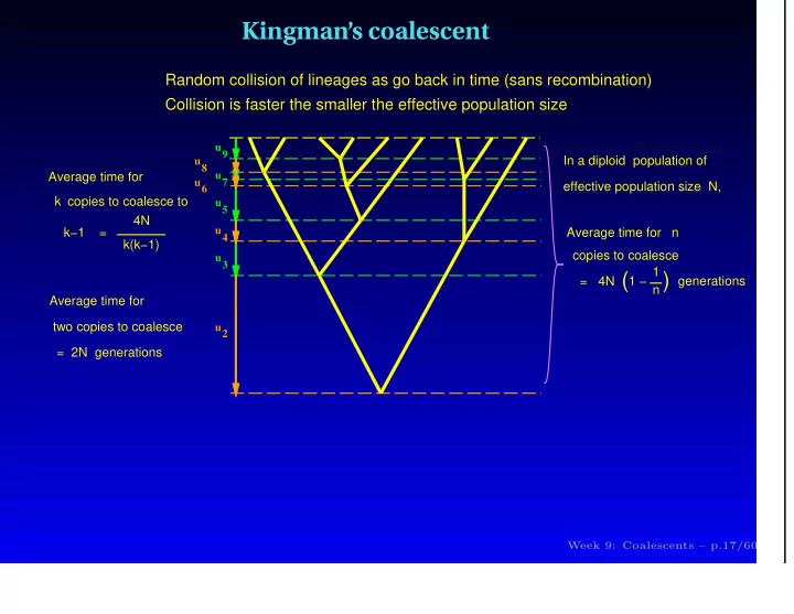
u9 u7 u5 u3 u8 u6 u4 u2

Random collision of lineages as go back in time (sans recombination) Collision is faster the smaller the effective population size

Average time for n Average time for copies to coalesce to 4N k(k−1) k−1 = In a diploid population of effective population size N, copies to coalesce = 4N (1 − 1 n

(

generations k Average time for two copies to coalesce = 2N generations

Week 9: Coalescents – p.17/60

SLIDE 2

Coalescence is faster in small populations

Change of population size and coalescents

Ne

time

the changes in population size will produce waves of coalescence

time

Coalescence events

time

the tree

The parameters of the growth curve for Ne can be inferred by likelihood methods as they affect the prior probabilities of those trees that fit the data.

Week 9: Coalescents – p.24/60

SLIDE 3

“Skyline” and “Skyride” plots in BEAST

Classical Skyline Plot

Effective Population Size

0.15 0.10 0.05 0.00 0.001 0.01 1.0 ORMCP Model 0.15 0.10 0.05 0.00 0.001 0.01 1.0 Bayesian Skyline Plot 0.15 0.10 0.05 0.00 0.001 0.01 1.0 Uniform Bayesian Skyride

Time (Past to Present) Effective Population Size

0.15 0.10 0.05 0.00 0.001 0.01 1.0 Time−Aware Bayesian Skyride

Time (Past to Present)

0.15 0.10 0.05 0.00 0.001 0.01 1.0 BEAST Bayesian Skyride

Time (Past to Present)

0.15 0.10 0.05 0.00 0.001 0.01 1.0

Figure from Minin, Bloomquist, and Suchard 2008

SLIDE 4

BEST Liu and Pearl (2007); Edwards et al. (2007)

X – sequence data
G – a genealogy (gene tree – with branch lengths)
S – a species tree
θ – demographic parameters
Λ – parameters of molecular sequence evolution

Pr(S, θ|X) = Pr(S, θ) Pr(X|S, θ) Pr(X) = Pr(S) Pr(θ)

Pr(X|G) Pr(G|S, θ)dG

∝ Pr(S) Pr(θ) Pr(X|G, Λ) Pr(Λ)dΛ

Pr(G|S, θ)dG

SLIDE 5

BEST – importance sampling

1. Generate

a collection

f

gene trees, G, using an approximation of the coalescent prior

2. Sample from the distribution of the species trees conditional
n the gene trees, G.
3. Use “importance weights” to correct the sample for the fact

that an approximate prior was used

SLIDE 6

BEST – importance sampling

1. Generate

a collection

f

gene trees, G, using an approximation of the coalescent prior (a) Use a tweaked version of MrBayes to sample N sets of gene trees, G, from

†

Pr(G|X) = Pr†(G) Pr(X|G) Pr†(X) (b) Pr†(G) is an approximate prior on gene trees from using a “maximal” species tree.

2. Sample from the distribution of the species trees conditional
n the gene trees, G.
3. Use “importance weights” to correct the sample for the fact

that an approximate prior was used

SLIDE 7

BEST – importance sampling

1. Generate

a collection

f

gene trees, G, using an approximation of the coalescent prior

2. Sample from the distribution of the species trees conditional
n the gene trees, G.

(a) From each set of gene trees (Gj for 1 ≤ j ≤ N) generate k species trees using coalescent theory: Pr(Si|Gj) = Pr(Si) Pr(Gj|Si) Pr(Gj)

3. Use “importance weights” to correct the sample for the fact

that an approximate prior was used

SLIDE 8

BEST – importance sampling

1. Generate a collection of gene trees, G, using an approximation of the

coalescent prior

2. Sample from the distribution of the species trees conditional on the gene

trees, G.

3. Use “importance weights” to correct the sample for the fact that an

approximate prior was used (a) Estimate Pr(Gj) by using the harmonic mean estimator from the MCMC in step 2. (b) Compute a normalization factor β =

N

j=1
Pr(Gj)

Pr(Gj) (c) Reweight all sampled species trees by

Pr(Gj)

Pr(Gj)β

SLIDE 9

BEST – conclusions

1. very expensive computationally (long MrBayes runs are

needed)

2. should correctly deal with the variability in gene tree caused

by the coalescent process.

SLIDE 10

∗BEAST overview

Goal: approximate Pr(S|X) Pr(S|X) ∝ Pr(X|S) Pr(S) =

Pr(X|G) Pr(G|S) Pr(S)dG

= Pr(X|G) Pr(G|S, θ) Pr(S)dGdθ = Pr(X|G, Λ) Pr(G|S, θ) Pr(S)dGdθdΛ θ = {N1, N2, . . . , } Λ = {κ, π, . . .}

SLIDE 11

Pr(S) from speciation model S

SLIDE 12

Pr(G|S) S G

SLIDE 13

Gene tree in a species tree w/ variable population size

Figure modified from Heled and Drummond 2010

A C B A1 A2 A3 C1 C2 C3 B2 B1 B3

Pr(G|S) = b

i Pr(Gi|Si)

G in grey S in black

SLIDE 14

In Species A

SLIDE 15

In Species C

SLIDE 16

In Species B

SLIDE 17

In ancestor of AC

SLIDE 18

In ancestor of ACB

SLIDE 19

Gene tree in a species tree w/ variable population size

Figure modified from Heled and Drummond 2010

A C B A1 A2 A3 C1 C2 C3 B2 B1 B3

Pr(G|S) = b

i Pr(Gi|Si)

G in grey S in black

SLIDE 20

MCMC update to gene tree

→

Changing G affects Pr(X|G, Λ) and Pr(G|S, θ)

SLIDE 21

Another MCMC update to gene tree

→

Some changes to G are incompatible with S (and will be rejected).

SLIDE 22

MCMC update to species tree

→

Changing S affects Pr(G|S, θ), but not Pr(X|G, Λ). Note that the red dots are “flags” for when a lineage enters a new species; the heights are determined by the species tree.

SLIDE 23

Another MCMC update to species tree

→

Some changes to S are incompatible with C (and will be rejected).

SLIDE 24

An MCMC update to the population size

→

Ne ∈ θ, so changing Ne affects Pr(G|S, θ), but not Pr(X|G, Λ).

SLIDE 25

Multiple gene tree in a species tree w/ variable population size

Figure from modified Heled and Drummond 2010

SLIDE 26

∗BEST

Similar model to BEST, but much more efficient implementation. Both attempt to sample the posterior distribution of species trees, gene trees, demographic parameter values and mutational parameter values. Both will be very sensitive to migration, but they represent the state-of-the-art for estimating species trees from gene trees.

SLIDE 27

Multiple Sequence Alignment - main points

The goal of MSA is to introduce gaps such that residues in

the same column are homologous (all residues in the column descended from a residue in their common ancestor).

The problem is recast as:

– reward matches (+ scores) – penalize rare substitutions (- scores), – penalize gaps (- scores), – try to find an alignment that maximizes the total score

pairwise alignment is tractable
MSA is usually done progressively
progressive alignment algorithms are heuristic, and do not
ptimize an evolutionary defensible criterion

SLIDE 28

Multiple Sequence Alignment tools

clustal variants are popular, but not very reliable.
simultaneous inference of MSA and tree is the most defensible

(but computationally demanding)

Promising tools for MSA (roughly in order of computational

tractability):

1. Simultaneous MSA + Trees (Handel, BAliPhy, BEAST,
AliFritz. . .)
2. FSA (fast statistical alignment); Infernal (for rRNA);

Prank

3. MAFFT, Muscle, ProbCons
Iterative

“meta-solutions” (e.g. SAT` e ) allow MSA uncertainty to be incorporated in tree inference.

GBlocks (and similar tools) cull ambiguously aligned regions.

SLIDE 29

human KRSV chimp KRV

rang

KPRV

SLIDE 30

KPSV KPRV KRSV KRV KRSV S->R del S P->R

human chimp orangutan

SLIDE 31

human KRSV chimp KRV gorilla KSV

rang

KPRV How should we align these sequences? human KRSV human KRSV chimp KR-V OR chimp K-RV gorilla KS-V gorilla K-SV

rang

KPRV

rang

KPRV

SLIDE 32

Pairwise alignment

Gap penalties and a substitution matrix imply a score for any alignment. Pairwise alignment involves finding the alignment that maximizes this score.

substitution matrices assign positive values to

matches or similar substitutions (for example Leucine→Isoleucine).

unlikely substitutions receive negative scores
gaps are rare and are heavily penalized (given large

negative values).

SLIDE 33

Scoring an alignment. Simplest case

Costs: Match 1 Mismatch Gap

5

Alignment:

Pongo V D E V G G E L G R L F V V P T Q Gorilla V E V A G D L G R L L I V Y P S R Score 1 1 1 1 1

Total score = 5

SLIDE 34

Scoring an different alignment. Simplest case

Match 1 Mismatch Gap

5

Pongo V D E V G G E L G R L

F

V V P T Q Gorilla V

E

V A G D L G R L L I V Y P S R Score 1

5

1 1 1 1 1 1 1

5

1 1

Total score = 0

SLIDE 35

BLOSUM 62 Substitution matrix

A R N D C Q E G H I L K M F P S T W Y V A 4 R

1

5 N

2

6 D

2
2

1 6 C

3
3
3

9 Q

1

1

3

5 E

1

2

4

2 5 G

2
1
3
2
2

6 H

2

1

1
3
2

8 I

1
3
3
3
1
3
3
4
3

4 L

1
2
3
4
1
2
3
4
3

2 4 K

1

2

1
3

1 1

2
1
3
2

5 M

1
1
2
3
1
2
3
2

1 2

1

5 F

2
3
3
3
2
3
3
3
1
3

6 P

1
2
2
1
3
1
1
2
2
3
3
1
2
4

7 S 1

1

1

1
1
2
2
1
2
1

4 T

1
1
1
1
1
2
2
1
1
1
1
2
1

1 5 W

3
3
4
4
2
2
3
2
2
3
2
3
1

1

4
3
2

11 Y

2
2
2
3
2
1
2
3

2

1
1
2
1

3

3
2
2

2 7 V

3
3
3
1
2
2
3
3

3 1

2

1

1
2
2
3
1

4 A R N D C Q E G H I L K M F P S T W Y V

SLIDE 36

Scoring an alignment with the BLOSUM 62 matrix

Pongo V D E V G G E L G R L F V V P T Q Gorilla V E V A G D L G R L L I V Y P S R Score 4 2

2

6

6
3
4
2
2

4 4

1

7 4 1

The score for the alignment is Dij =

k

d(k)

ij

If i indicates Pongo and j indicates Gorilla Dij = 12

SLIDE 37

Scoring an alignment with gaps

If the GP is -8:

Pongo V D E V G G E L G R L

F

V V P T Q Gorilla V

E

V A G D L G R L L I V Y P S R Score 4

8

5 5 6 2 4 6 5 4

8

4

1

7 4 1

By introducing gaps we have improved the score: Dij = 40

SLIDE 38

Gap Penalties

Gaps are penalized more heavily than substitutions to avoid alignments like this: Pongo VDEVGGE-LGRLFVVPTQ Gorilla VDEVGG-WLGRLFVVPTQ

SLIDE 39

Gap Penalties

Because multiple residues are often inserted or deleted at the same time, affine gap penalties are

ften used:

GP = GO + lGE where:

GP is the gap penalty.
GO is the “gap-opening penalty”
GE is the “gap-extension penalty”
l is the length of the gap

SLIDE 40

Finding an optimal alignment

V E V A G D L G R L L I Y P S R V V E D E V G G L G V R L F V P T Q

Pongo Gorilla

SLIDE 41

Aligning two sequences, each with length = 1

D

→ •

E ↓ ց ↓

→ •

SLIDE 42

Alignment 1

D

→
D-

E ↓ ց ↓

E
→

SLIDE 43

Alignment 2

D

→
D

E ↓ ց ↓ E

→

SLIDE 44

Alignment 3

D

→
D

E ↓ ց ↓ E-

→

SLIDE 45

Longer sequences – up to 2 amino acids!

V D

→ • → •

V ↓ ց ↓ ց ↓

→ •

→ • E ↓ ց ↓ ց ↓

→ •

→ •

SLIDE 46

Alignment 1

V D

→ • → •

V ↓ ց ↓ ց ↓ VD--

→ •

→ •

-VE

E ↓ ց ↓ ց ↓

→ •

→ •

SLIDE 47

Alignment 2

V D

→ • → •

V ↓ ց ↓ ց ↓ VD-

→ •

→ •

VE

E ↓ ց ↓ ց ↓

→ •

→ •

SLIDE 48

Alignment 3

V D

→ • → •

V ↓ ց ↓ ց ↓ V-D-

→ •

→ •

V-E

E ↓ ց ↓ ց ↓

→ •

→ •

SLIDE 49

Alignment 4

V D

→ • → •

V ↓ ց ↓ ց ↓ V-D

→ •

→ •

VE

E ↓ ց ↓ ց ↓

→ •

→ •

SLIDE 50

Alignment 5

V D

→ • → •

V ↓ ց ↓ ց ↓ V--D

→ •

→ •

VE-

E ↓ ց ↓ ց ↓

→ •

→ •

SLIDE 51

Alignment 6

V D

→ • → •

V ↓ ց ↓ ց ↓ VD-

→ •

→ • V-E E ↓ ց ↓ ց ↓

→ •

→ •

SLIDE 52

Alignment 7

V D

→ • → •

V ↓ ց ↓ ց ↓ VD

→ •

→ • VE E ↓ ց ↓ ց ↓

→ •

→ •

SLIDE 53

Alignment 8

V D

→ • → •

V ↓ ց ↓ ց ↓ V-D

→ •

→ • VE- E ↓ ց ↓ ց ↓

→ •

→ •

SLIDE 54

Alignment 9

V D

→ • → •

V ↓ ց ↓ ց ↓

VD-
→ •

→ • V--E E ↓ ց ↓ ց ↓

→ •

→ •

SLIDE 55

Alignment 10

V D

→ • → •

V ↓ ց ↓ ց ↓

VD
→ •

→ • V-E E ↓ ց ↓ ց ↓

→ •

→ •

SLIDE 56

Alignment 11

V D

→ • → •

V ↓ ց ↓ ց ↓

V-D
→ •

→ • V-E- E ↓ ց ↓ ց ↓

→ •

→ •

SLIDE 57

Alignment 12

V D

→ • → •

V ↓ ց ↓ ց ↓

VD
→ •

→ • VE- E ↓ ց ↓ ց ↓

→ •

→ •

SLIDE 58

Alignment 13

V D

→ • → •

V ↓ ց ↓ ց ↓

-VD
→ •

→ • VE-- E ↓ ց ↓ ց ↓

→ •

→ •

SLIDE 59

Pongo V D E V G G E L G R L F V V P T Q Gorilla V E V A G D L G R L L I V Y P S R Score 4 2

2

6

6
3
4
2
2

4 4

1

7 4 1

V E V A G D L G R L L I Y P S R V V E D E V G G L G V R L F V P T Q

Pongo Gorilla

SLIDE 60

Pongo V D E V G G E L G R L

F

V V P T Q Gorilla V

E

V A G D L G R L L I V Y P S R Score 4

8

5 5 6 2 4 6 5 4

8

4

1

7 4 1

V E V A G D L G R L L I Y P S R V V E D E V G G L G V R L F V P T Q

Pongo Gorilla

SLIDE 61

length Seq # 1 length Seq # 2 # alignments 1 1 3 2 2 13 3 3 63 4 4 321 5 5 1,683 6 6 8,989 7 7 48,639 8 8 265,729 9 9 1,462,563 . . . . . . . . . 17 17 1,425,834,724,419

SLIDE 62

Needleman-Wunsch algorithm (paraphrased)

Work from the top left (beginning of both sequences)
For each cell store the highest score possible for that cell

and a “back” pointer to tell point to the previous step in the best path

When you reach the lower right corner, you know the optimal

score and the back pointers tell you the alignment. The highest-score calculation at each cell only depends on its the cell’s three possible previous neighbors. If one sequence is length N, and the other is length M, then Needleman-Wunsch only takes ≈ 6NM calculations. But there are a much larger number of possible alignments.

SLIDE 63

V D E V G G

V
E
V
A
G
D

SLIDE 64

V D E V G G ←

5
V

↑

5
E
V
A
G
D

SLIDE 65

V D E V G G ←

5

←

10
V

↑ տ

5

4

E

↑

10
V
A
G
D

SLIDE 66

V D E V G G ←

5

←

10

←

15
V

↑ տ

5

4 ←

1
E

↑ ↑

10
1
V

↑

15
A
G
D

SLIDE 67

V D E V G G ←

5

←

10

←

15

←

20
V

↑ տ

5

4 ←

1

←

6
E

↑ ↑ տ

10
1

6

V

↑ տ ↑

15
6
A

↑

20
G
D

SLIDE 68

V D E V G G ←

5

←

10

←

15

←

20

←

25
V

↑ տ

5

4 ←

1

←

6

←

11
E

↑ ↑ տ տ

10
1

6 4

V

↑ տ ↑ ↑

15
6

1

A

↑ ↑

20
11
G

↑

25
D

SLIDE 69

V D E V G G E L G R ←

5

←

10

←

15

←

20

←

25

←

30

←

35

←

40

←

45

←

50

V ↑ տ տ

5

4 ←

1

←

6
11

←

16

←

21

←

26

←

31

←

36

←

41

E ↑ ↑ տ տ տ

10
1

6 4 ←

1

←

6

←

11
16

←

21

←

26

←

31

V ↑ տ ↑ տ տ

15
6

1 4 8 ← 3 ←

2

←

7

←

12

←

17

←

22

A ↑ ↑ ↑ տ տ տ տ տ

20
11
4

4 8 3 ←

2

←

7
12

←

17

G ↑ ↑ ↑ ↑ ↑ տ տ տ

25
16
9
5
1

10 14 ← 9 ← 4

1

←

6

D ↑ ↑ տ տ ↑ ↑ տ տ

30
21
10
7
6

5 9 16 ← 11 ← 6 ← 1 L ↑ ↑ ↑ ↑ տ ↑ ↑ ↑ տ

35
26
15
12
6

4 11 20 ← 15 ← 10 G ↑ ↑ ↑ տ ↑ տ տ ↑ ↑ տ

40
31
20
17
11

6 6 15 26 ← 21 R ↑ ↑ ↑ տ ↑ ↑ ↑ տ ↑ ↑ տ

45
36
25
20
16
5

1 6 10 21 31 L ↑ ↑ ↑ ↑ տ ↑ ↑ ↑ տ ↑ ↑

50
41
30
25
19
10
4

1 10 16 26 L ↑ ↑ ↑ ↑ տ ↑ ↑ ↑ տ ↑ ↑

55
46
35
30
24
15
9
4

5 11 21 I ↑ ↑ ↑ ↑ տ ↑ ↑ ↑ ↑ ↑ ↑

60
51
40
35
27
20
14
9

6 16 V ↑ տ ↑ ↑ տ ↑ ↑ ↑ ↑ ↑ ↑

SLIDE 70

SLIDE 71

Aligning multiple sequences

B D A C E

SLIDE 72

Progressive alignment

Devised by Feng and Doolittle 1987 and Higgins and Sharp, 1988. An approximate method for producing multiple sequence alignments using a guide tree.

Perform pairwise alignments to produce a distance matrix
Produce a guide tree from the distances
Use the guide tree to specify the ordering used for aligning sequences,

closest to furthest.

SLIDE 73

A PEEKSAVTALWGKVN--VDEVGG B GEEKAAVLALWDKVN--EEEVGG C PADKTNVKAAWGKVGAHAGEYGA D AADKTNVKAAWSKVGGHAGEYGA E EHEWQLVLHVWAKVEADVAGHGQ A - B .17 - C .59 .60 - D .59 .59 .13 - E .77 .77 .75 .75 -

A B D C E

A PEEKSAVTALWGKVNVDEVGG B GEEKAAVLALWDKVNEEEVGG C PADKTNVKAAWGKVGAHAGEYGA E EHEWQLVLHVWAKVEADVAGHGQ D AADKTNVKAAWSKVGGHAGEYGA A PEEKSAVTALWGKVNVDEVGG B GEEKAAVLALWDKVNEEEVGG C PADKTNVKAAWGKVGAHAGEYGA E EHEWQLVLHVWAKVEADVAGHGQ D AADKTNVKAAWSKVGGHAGEYGA +

tree inference pairwise alignment alignment stage

SLIDE 74

Alignment stage of progressive alignments Sequences of clades become grouped into “profiles” as the algorithm descends the tree. The next youngest internal nodes is selected at each step to create a new profile. Alignment at each step involves

Sequence-Sequence
Sequence-Profile
Profile-Profile

SLIDE 75

Aligning multiple sequences

B D A C E

Seq-Seq Seq-Seq Seq-Profile Profile-Profile

0.1 0.1 0.2 0.12 0.09 0.15 0.27 .1

SLIDE 76

Profile to Profile alignment

V E V A G D L G R L L I Y P S R A V E D E V G G L G M R L F V P T Q L D D E V - G A G V R L F V P T Q V E I A G D L

L

L L Y P T R V V E V A G E L

L

L L Y P T K I

SLIDE 77

Profile to profile alignments Adding a gap to a profile means that every member of that group of sequences gets a gap at that position of the sequence. Usually the scores for each edge in the Needleman-W¨ unsch graph are calculated using a “sum of pairs” scoring system. clustal W1 uses weights assigned to each sequence in a profile group to downweight closely related sequences so that they are not overrepresented.

1Thompson, Higgins, and Gibson. Nuc. Acids. Res. 1994

SLIDE 78

Profile 1 Profile 2 Seq weight AA taxon A 0.3 V taxon C 0.24 A taxon E 0.19 I Seq weight AA taxon B 0.15 V taxon D 0.25 M DP 1,P 2 =

i
j wiwjdij

ninj = 1 6 [d(V, V )wAwB + d(V, M)wAwD + d(A, V )wCwB . . . = . . . d(A, M)wCwD + d(I, V )wEwB + d(I, M)wEwD] = 1 6(4 × 0.3 × 0.15 + 1 × 0.3 × 0.25 + 0 × 0.24 × 0.15 . . . = . . . −1 × 0.24 × 0.25 + 3 × 0.19 × 0.15 + 1 × 0.19 × 0.15) = 1.46225

SLIDE 79

Dealing with alignment ambiguity2

X Y Z 1 2 3 4 5 6 7 8 9 1 1 1 0 1 2 Outgroup T A G A G C A C T C A G Taxon A T A G A G C A C T C A G Taxon B T A G T G A A G C C A G Taxon C T A G T G A A G C C A G Taxon D T A G A G C C A G Taxon E T A G A G C C A G

(a)

X Y Z 1 2 3 4 5 6 7 8 9 1 1 1 0 1 2 Outgroup T A G A G C A C T C A G Taxon A T A G A G C A C T C A G Taxon B T A G T G A A G C C A G Taxon C T A G T G A A G C C A G Taxon D T A G A G C - - - C A G Taxon E T A G A G C - - - C A G

(b) (c)

X Y Z 1 2 3 4 5 6 7 8 9 1 1 1 0 1 2 Outgroup T A G A G C A C T C A G Taxon A T A G A G C A C T C A G Taxon B T A G T G A A G C C A G Taxon C T A G T G A A G C C A G Taxon D T A G - - - A G C C A G Taxon E T A G - - - A G C C A G

2from M. S. Y. Lee, TREE, 2001

SLIDE 80

Dealing with alignment ambiguity3 - deletion

X Y Z 1 2 3 4 5 6 7 8 9 1 1 1 0 1 2 Outgroup T A G A G C A C T C A G Taxon A T A G A G C A C T C A G Taxon B T A G T G A A G C C A G Taxon C T A G T G A A G C C A G Taxon D T A G A G C C A G Taxon E T A G A G C C A G

(a)

X Z 1 2 3 1 1 1 0 1 2 Outgroup T A G C A G Taxon A T A G C A G Taxon B T A G C A G Taxon C T A G C A G Taxon D T A G C A G Taxon E T A G C A G X Y Z 1 2 3 4 5 6 7 8 9 1 1 1 0 1 2 Outgroup T A G A G C A C T C A G Taxon A T A G A G C A C T C A G Taxon B T A G T G A A G C C A G Taxon C T A G T G A A G C C A G Taxon D T A G ? ? ? - - - C A G Taxon E T A G ? ? ? - - - C A G

3from M. S. Y. Lee, TREE, 2001

SLIDE 81

Dealing with alignment ambiguity4 Elision method (Wheeler, 1995) involves simply concatenating matrices.

(e)

X Y Z 1 2 3 4 5 6 7 8 9 1 1 1 0 1 2 Outgroup T A G A G C A C T C A G Taxon A T A G A G C A C T C A G Taxon B T A G T G A A G C C A G Taxon C T A G T G A A G C C A G Taxon D T A G - - - A G C C A G Taxon E T A G - - - A G C C A G X Y Z 1 2 3 4 5 6 7 8 9 1 1 1 0 1 2 T A G A G C A C T C A G T A G A G C A C T C A G T A G T G A A G C C A G T A G T G A A G C C A G T A G A G C - - - C A G T A G A G C - - - C A G

4from M. S. Y. Lee, TREE, 2001

SLIDE 82

Simultaneous tree inference and alignment

Ideally we would address uncertainty in both types of

inference at the same time

Allows for application of statistical models to improve

inference and assessments of reliability

Just now becoming feasible:

POY (Wheeler, Gladstein, Laet, 2002), Handel (Holmes and Bruno, 2001), BAliPhy (Redelings and Suchard, 2005), and BEAST(Lunter et al., 2005, Drummond and Rambaut, 2003). SATe (Liu et al 2009; Yu and Holder software).

SLIDE 83

References Edwards, S. V., Liu, L., and Pearl, D. K. (2007). High- resolution species trees without concatenation. Proceedings

f the National Academy of Sciences, 104(14):5936–5941.

Liu, L. and Pearl, D. K. (2007). Species trees from gene trees: reconstruction Bayesian posterior distributions of a species phylogeny using estimated gene tree distributions. Systematic Biology, 56(3):504–514.