Introduction to Machine Learning Classification: Naive Bayes - - PowerPoint PPT Presentation

introduction to machine learning classification naive
SMART_READER_LITE
LIVE PREVIEW

Introduction to Machine Learning Classification: Naive Bayes - - PowerPoint PPT Presentation

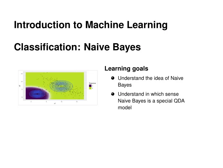
Introduction to Machine Learning Classification: Naive Bayes Learning goals 15 Understand the idea of Naive 10 Response Bayes x2 a b 5 Understand in which sense 0 Naive Bayes is a special QDA 0 5 10 15 x1 model NAIVE BAYES


slide-1
SLIDE 1

Introduction to Machine Learning Classification: Naive Bayes

5 10 15 5 10 15 x1 x2 Response a b

Learning goals

Understand the idea of Naive Bayes Understand in which sense Naive Bayes is a special QDA model

slide-2
SLIDE 2

NAIVE BAYES CLASSIFIER

NB is a generative multiclass technique. Remember: We use Bayes’ theorem and only need p(x|y = k) to compute the posterior as:

πk(x) = P(y = k | x) = P(x|y = k)P(y = k) P(x) =

p(x|y = k)πk

g

  • j=1

p(x|y = j)πj NB is based on a simple conditional independence assumption: the features are conditionally independent given class y. p(x|y = k) = p((x1, x2, ..., xp)|y = k) =

p

  • j=1

p(xj|y = k). So we only need to specify and estimate the distribution p(xj|y = k), which is considerably simpler as this is univariate.

c

  • Introduction to Machine Learning – 1 / 5
slide-3
SLIDE 3

NB: NUMERICAL FEATURES

We use a univariate Gaussian for p(xj|y = k), and estimate (µj, σ2

j ) in

the standard manner. Because of p(x|y = k) =

p

  • j=1

p(xj|y = k), the joint conditional density is Gaussian with diagonal but non-isotropic covariance structure, and potentially different across classes. Hence, NB is a (specific) QDA model, with quadratic decision boundary.

5 10 15 5 10 15

x1 x2 Response

a b

c

  • Introduction to Machine Learning – 2 / 5
slide-4
SLIDE 4

NB: CATEGORICAL FEATURES

We use a categorical distribution for p(xj|y = k) and estimate the probabilities pkjm that, in class k, our j-th feature has value m, xj = m, simply by counting the frequencies. p(xj|y = k) =

  • m

p[xj=m]

kjm

Because of the simple conditional independence structure it is also very easy to deal with mixed numerical / categorical feature spaces.

c

  • Introduction to Machine Learning – 3 / 5
slide-5
SLIDE 5

LAPLACE SMOOTHING

If a given class and feature value never occur together in the training data, then the frequency-based probability estimate will be zero. This is problematic because it will wipe out all information in the other probabilities when they are multiplied. A simple numerical correction is to set these zero probabilities to a small value to regularize against this case.

c

  • Introduction to Machine Learning – 4 / 5
slide-6
SLIDE 6

NAIVE BAYES: APPLICATION AS SPAM FILTER

In the late 90s, Naive Bayes became popular for e-mail spam filter programs Word counts were used as features to detect spam mails (e.g., "Viagra" often occurs in spam mail) Independence assumption implies: occurrence of two words in mail is not correlated Seems naive ("Viagra" more likely to occur in context with "Buy now" than "flower"), but leads to less required parameters and therefore better generalization, and often works well in practice.

c

  • Introduction to Machine Learning – 5 / 5