Introduction Ryan Martin UIC www.math.uic.edu/~rgmartin 1 Based on - - PowerPoint PPT Presentation

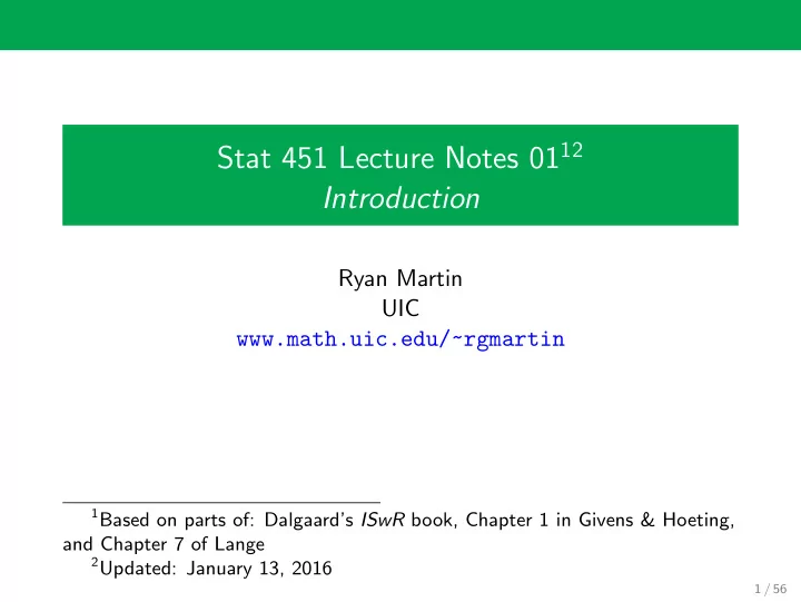
Stat 451 Lecture Notes 0112 Introduction

Ryan Martin UIC www.math.uic.edu/~rgmartin

1Based on parts of: Dalgaard’s ISwR book, Chapter 1 in Givens & Hoeting,

and Chapter 7 of Lange

2Updated: January 13, 2016 1 / 56

What to compute?

Stat 451 is a course about computational statistics. Therefore, it is important first to discuss what we want to compute in a statistics problems. Here, we are basically concerned with two kinds of things:

maximizing the likelihood function integrating a “posterior distribution”

The former notion should be familiar from your experience with maximum likelihood in Stat 411. The latter may be new to you — it’s “Bayesian”. Next is a brief introduction to these concepts, along with a non-trivial illustration.

2 / 56

Maximum likelihood

Suppose we have n independent observations, Y1, . . . , Yn, and the density/mass function pθ for these observations depends

• n an unknown parameter θ.

The likelihood and log-likelihood functions are L(θ) =

n

• i=1

pθ(Yi) and ℓ(θ) =

n

• i=1

log pθ(Yi). The maximum likelihood estimator (MLE) ˆ θ of θ, based on data, maximizes the likelihood, i.e., ˆ θ = arg max

θ

L(θ) ⇐ ⇒ ˙ ℓ(ˆ θ) = 0. Need to be able to optimize and/or find roots of functions.

3 / 56

Maximum likelihood (cont)

Besides producing an estimate of the unknown parameter, we might also like to assess its uncertainty. In Stat 411 you learn that, under some conditions, when the sample size n is large, the distribution of ˆ θ is approximately normal with mean θ and variance I(θ)−1, where I(θ) is the Fisher information matrix: I(θ) = Eθ{ ˙ ℓ(θ) ˙ ℓ(θ)⊤} = −Eθ{¨ ℓ(θ)}. Then an approximate 95% confidence interval for θj is ˆ θj ± 1.96 ·

• [I(ˆ

θ)−1]jj, j = 1, . . . , d. So, computing derivatives and inverting matrices is important.

4 / 56

Bayesian approach

The Bayesian approach is based on using the rules of probability for inference. Start with a prior distribution for θ, with density/mass function π(θ), basically just a weight function. Yields a conditional distribution for θ, given Y , as π(θ | Y ) = L(θ)π(θ)

• L(u)π(u) du ∝ L(θ)π(θ).

Now we treat π(θ | Y ) as the object of interest and the goal is to produce various summaries, such as mean, variance, quantiles, probabilities, etc. So, integrating functions will be important.

5 / 56

Example: probit regression

Y1, . . . , Yn are independent (not iid) binary observations. Specifically, Yi

ind

∼ Ber

• Φ(x⊤

i θ)

• , i = 1, . . . , n, where:

“Ber” denotes a Bernoulli distribution; x1, . . . , xn are fixed d-dimensional covariates; θ is a d-dimensional parameter vector; and Φ is the standard normal distribution function.3

Exercise:

write out log-likelihood function calculate Fisher information matrix ...

3Other cdfs can be used, but then the model isn’t called “probit”... 6 / 56

Remarks

This course will mainly study how to solve certain optimization and integration problems that arise in statistics applications. We’ll need some background on general numerical methods. Software will also be important — we will use R. Some of what we discuss in the class will be simple, other things more difficult. My goal is that students completing the course will have sufficient background to read current papers on computational statistics and implement their methods.

7 / 56

Outline

1 Review of statistical inference 2 Introduction to R Basics R session R graphics R programming Data entry 3 Math and stat tools

8 / 56

General facts about R

R is a free version of the S-PLUS software. Can be downloaded for free (http://cran.r-project.org) for Windows, Mac, and Unix computers. Environment is interactive by default—like a calculator—but users can create files of R code (called scripts) on the side which can be run all at once within R. It is possible to write code that works together with lower-level programming languages like C and FORTRAN (for speed). R is powerful because of its flexibility — users can easily define their own functions or modify existing functions to suit their needs.

9 / 56

Arithmetic

Among other things, R can do arithmetic like a calculator. Basic binary (arithmetic) operations are: + Addition ^ or ** Exponentiation

• Subtraction

%/% Integer division * Multiplication %% Modulus (remainder) / Division

10 / 56

Variables and assignments

Even with fairly routine calculations it is helpful to be able to store some intermediate values. R allows users to assign a value to a particular variable. Syntax: x <- 7 This means that the value 7 is assigned to the variable x. Note: The assignment symbol <- is to be treated as a single character, an arrow pointing to the left. One can use the underscore symbol or an equal sign in place

• f the assignment character — not recommended.

Underscore symbol cannot be used in variable names; use a period instead, e.g., pred.value.

11 / 56

Expressions and objects

In R, the user enters an expression and the system evaluates it and produces output. These expressions need not be formulas — they can generate graphs, output data sets, etc. Expressions work on objects, basically anything that can be assigned to a variable. But the syntax used is expression/object specific. In what follows we will discuss several important types of expressions and objects. Use the str(X) to view the “structure” of the object X.

12 / 56

Functions and arguments

Functions in R can take many forms:

There’s the kind that look like mathematical functions, say log(x), and the kind that don’t, say plot(x, y, pch=2).

The common feature is that there is a set of parantheses containing those arguments that the fuction applies to. Two “types” of arguments:

Positional – variable recognized by position in the list. Named – variable recognized by name.

Some functions don’t have arguments, some have default arguments, and some allow “arbitrary” arguments. R has an extensive list of built-in function that can do all sorts

• f things – and it’s easy to write your own functions since the

function syntax in R is the same as ordinary R syntax.

13 / 56

Vectors

Numeric vectors are fairly straightforward. There are basically4 two other kinds of vectors:

Character Logical

Character vectors have elements made up of character strings; e.g. names <- c(’Small’, ’Medium’, ’Large’) Logical vectors have elements TRUE or FALSE, and are very useful for indexing data sets. An example of how to get a logical vector: > gpa <- c(3.0, 2.8, 3.4, 3.7, 3.9, 3.3) > gpa > 3.5 [1] FALSE FALSE FALSE TRUE TRUE FALSE

4Complex vectors also exist 14 / 56

Vectors (cont.)

Three functions to create vectors:

c() – concatenate seq() – patterned sequence rep() – repeat something

A vector must contain elements of the same “type”, so what happens if two variables x and y of different types are concatenated? The general (and non-informative) answer is that they are coerced into types that match. For example: > c(FALSE, 7) [1] 0 7 > c(11.7, ’abc’) [1] ’11.7’ ’abc’

15 / 56

Vectors (cont.)

An interesting feature of R is that it does “vectorized arithmetic.” That is, R will apply arithmetic operations (and some other functions) in a natural way. For example: > x <- c(7, 10, 11) > y <- seq(5, 3, by=-1) > x + y [1] 12 14 14 If the two vectors are not of the same length, the shorter one gets “recycled” — error message if the length of the longer vector is not a multiple of the length of the shorter vector. When defining your own functions, remember to be careful about assuming it will vectorize how you want it to!

16 / 56

Matrices and arrays

A natural extension of a vector is a matrix, which is just a vector with a double index. Example: M <- matrix(1:6, nrow=3, ncol=2). In R, matrices are almost always5 treated just like vectors. rbind() and cbind() functions can be used to append two

• r more matrices by rows and columns, respectively.

Can name the rows and columns with rownames() and colnames() functions. More generally, R can work with an array (a vector with n indices), but these are a bit less common, perhaps because they’re hard to visualize.

5The only time R treats matrices in a linear algebra sort of way is when the

user asks R to do something “linear algebra like” such as matrix multiplication.

17 / 56

Data frames

A data frame is R’s version of what we think of as a data matrix or data set. The columns represent variables and the rows represent cases. This idea is similar to a matrix, but matrices must be entirely

• f the same type, while data frames can have a mixture of

numeric, character, and logical variables. To create a data frame: D <- data.frame(list-of-variables) We’ll talk about reading files into a data frame later. Many statistical routines in R (e.g., linear regression) are designed to operate on data frames.

18 / 56

Lists

The list structure is quite different and (as far as I know) unique to R. A list in R is exactly as its name suggests — a list of objects. The distinguishing feature is that a list can contain (almost?) any kind of object in R. For example, objects in the list can be vectors, matrices, and even functions. Syntax: mylist <- list(list-of-objects). For example: > M <- matrix(c(2, 5, 7, 7), nrow=2) > f <- function(x) log(x)+x^2 > mylist <- list(mymat=M, myfun=f) > mylist$myfun(mylist$mymat)

19 / 56

Indexing

Given a vector/matrix/array/data frame/list, we would like to be able to pick off certain values. Need understand how these objects are indexed. For example, if M is a matrix, then M[i,j] refers to the value in the i-th row and j-th column of M. Also, M[,j] returns the j-th column of M as a vector. Data frames are indexed similarly, and vectors are just

• ne-dim matrices.

We’ve seen that objects of a list are indexed by their name and a $ sign. Example: What is mylist$mymat[2,2]? Example: What is mymat[-1,]?

20 / 56

Subsetting

By thinking of indexing in terms of logical variables, we can extend this idea to allow for subsetting of our object. For example, consider the code M[1,2].

This is equivalent to defining two logical vectors: > row.log <- (1:nrow(M)) == 1 > col.log <- (1:ncol(M)) == 2 Then M[1,2] is equivalent to M[row.log, col.log].

To generalize, we can define any sort of logical variable we like and apply it as above. For example, suppose a data frame D has a variable age. To get only those rows for adults, use the code D[,D$age > 19] There’s another generalization of the row/column indexing: > x <- seq(5, 25, by=5) > x[c(2,3)] [1] 10 15

21 / 56

Implicit loops

In many cases, we want to obtain some kind of summary of the rows and/or columns of a matrix or data frame (or list). Such a process requires scanning the particular dimension of the object and applying the function each time. R functions apply() and its variations do this directly. For lists, use lapply() or sapply(); for matrices or data frames use apply(). Syntax: Suppose x and y are two numeric vectors. > mylist <- list(var1=x, var2=y) > lapply(mylist, mean) > sapply(mylist, mean) > mymat <- cbind(var1=x, var2=y) > apply(mymat, 2, mean, na.rm=TRUE)

22 / 56

Sorting

Sorting a single vector is easy — use sort(x). But what if you want to sort the rows of a matrix by a particular column? Goal is to sort the rows data frame D by column 1. Use the order() function: > o <- order(D[,1]) > D.sorted <- D[o,] Using o <- order(D[,1], D[,2]) would sort D by the first column and then the second.

23 / 56

Outline

1 Review of statistical inference 2 Introduction to R Basics R session R graphics R programming Data entry 3 Math and stat tools

24 / 56

Workspace and directories

When you fire up R, you’ll have a working directory. To view this directory, type getwd(). Change the directory by typing setwd(’mydir’). To view the objects in the workspace, type ls(). To remove an object X from workspace, type rm(X).

25 / 56

Workspace and directories (cont.)

Save workspace to the working directory: save.image(). This command saves all the objects in the current workspace to a file .Rdata in the working directory — you can specify a different filename if you like. To save objects x, y and z in file myfile.Rd, type save(x, y, z, file=’myfile.Rd’) Load the saved file: load(file=’myfile.Rd’) Note: Saving the workspace does not save the output!

26 / 56

Saving input and output

The save command saves objects in the workspace, but does not save either the R input or output. R input (commands) can be stored in an external file, called a script, say myscript.R. Run commands in script: source(’myscript.R’). To begin a session where the output is stored in a file myfile, type sink(’myfile’). When an expression is evaluated, nothing is printed to the

• utput terminal — instead, everything is printed to the file

myfile until the user types sink().

27 / 56

Getting help

In R, type help(mean) to see some documentation for the function mean. You can also type ?mean for short. Typing help.start(’mean’) will open a HTML help file with searching capabilities, etc. Google searches are very helpful too. Extensive documentation online or in your installation — see “Introduction to R” and “Writing R Extensions” (probably more than you’ll ever need to know about R).

28 / 56

Packages

Thousands of extra packages are available that contain specialized functions and data sets. These functions often contain compiled (C or Fortran) code. Look at the CRAN repository for a list (with descriptions) of available packages. To install a package pkg, type install.packages(’pkg’) and follow the instructions. Once the package is installed, to access its contents type library(pkg). The objects within this package are now available for use.

29 / 56

Outline

1 Review of statistical inference 2 Introduction to R Basics R session R graphics R programming Data entry 3 Math and stat tools

30 / 56

Introduction

One of the main advantages of R is its graphical capabilities. This includes having a number of built-in graphical procedures, as well as giving the user the flexibility to produce his/her own plots. Here we’ll see a few examples of the available graphical tools, with some focus on how to annotate graphs for presentation. Note: It is possible to directly produce PDF or Postscript graphics for inclusion in LaTeX files.

31 / 56

Scatterplots

The following code contains lots of new ideas. Take notice of where the labels are printed! x <- runif(50, 0, 2) y <- runif(50, 0, 2) plot(x, y, xlab=’x-label’, ylab=’y-label’, main=’Main Title’, sub=’subtitle’) text(0.6, 0.6, ’text at (0.6,0.6)’) abline(h=0.6, v=0.6, lty=2) for(s in 1:4) mtext(-1:4, side=s, at=0.7, line=-1:4) mtext(paste(’side’, 1:4), side=1:4, line=-1, font=2)

32 / 56

Histograms

Histograms are very easy in R. The basic command is hist(X), where X is the variable you want to draw the histogram of. There are a number of options to customize this plot. You can add lines to the plot with curve(). Add a legend to label the various curves. See the mean.med.hist function in the code online.

33 / 56

Boxplots

Nice way to visualize the location and spread of a distribution. Especially useful for comparing two or more distributions. Basic syntax is boxplot(X) where X is a numeric vector or a list that contains multiple numeric vectors. Can do some similar sorts of customization. See the function mean.med.comp in the code online.

34 / 56

Outline

1 Review of statistical inference 2 Introduction to R Basics R session R graphics R programming Data entry 3 Math and stat tools

35 / 56

Flow control 1: If-then-else

An important part of programming is conditional execution of commands, and this is accomplished through the if-then-else structure. Basic syntax:

if(condition1) { ## Do something } else if(condition2) { ## Do something else } else { ## Do another thing }

Inside the if() is a logical variable, taking values TRUE or FALSE. Logical variables can be “combined” with the usual Boolean

• perators: & (and), | (or), ! (not).

To compare two variables, type A == B or A != B.

36 / 56

Flow control 2: Loops

The three major players are for(), while(), and repeat. Illustrate while() and repeat with an example of computing the square root of a non-negative number.

y <- 12345 x <- y / 2 while(abs(x*x - y) > 1e-10) x <- (x + y / x) / 2 print(x) # based on while() x <- y / 2 repeat { x <- (x + y / x) / 2 if(abs(x*x - y) < 1e-10) break } print(x) # based on repeat

37 / 56

Flow control 2: Loops (cont.)

The for() loop is by far the most common looping structure. It is typical to run the loop with a counter, stopping once the counter reaches it maximum value: for(i in 1:n) { ## Do something } In particular: x <- seq(0, 1, by=0.05) plot(x, x, type=’’l’’) for(j in 2:5) lines(x, x^j) But there’s a bunch of other things one can do too; e.g., for(i in (1:10)^4) for(j in c(2,5,7)) for(var in names(data)) for(f in c(sin, cos, tan))

38 / 56

Avoiding loops

Knowing when (and how) to avoid loops is as important as knowing how to use them. Loops are very easy to program in R, but can run very slow depending on the application. Often a version of the apply function is better. Example: find the maximum value in each column of X

Do this max.X <- apply(X, 2, max) don’t do this max.X <- rep(NA, ncol(X)) for(j in 1:ncol(X)) max.X[j] <- max(X[,j])

apply is sometimes much faster, other times not much faster; but it’s always much cleaner!

39 / 56

Outline

1 Review of statistical inference 2 Introduction to R Basics R session R graphics R programming Data entry 3 Math and stat tools

40 / 56

Reading data 1: scan

Aside from typing in data directly with c(...), the simplest way to read in data is with the scan command. Can read in vector or list objects. If file.dat is a text file containing numeric or character data, typing X <- scan(file=’file.dat’) will read the data from this file and store it in the vector X. Lists can also be done but the syntax is weird; go to help(scan) for details.

41 / 56

Reading data 2: read.table

In statistical applications, we usually have several variables measured on a number of cases. In such cases, a data frame is the most convenient data type. By default, R looks for data points arranged in columns with a single space separating two values.6 If two spaces (delimiters) appear next to one another, R assumes the value is missing, and enters NA. Suppose we have a file data.dat that contains data points separated by commas, with a header row containing the variable names. Then the syntax is

read.table(file=’data.dat’, header=TRUE, sep=’,’)

6It’s easy to change this default! 42 / 56

Reading data 2: read.table (cont.)

Things to consider when reading a file:

header line separator/delimiter quotes missing values unfilled lines white space in character fields comments ...

Check out help(read.table) for details. There are also some special shortcut functions, such as read.csv and read.delim, that read comma and tab delimited data files by default.

43 / 56

Writing data to a file

In some cases we will have an output data set that we would like to write to a file, perhaps for someone else using a different software to analyze. For a “rectangular” data object X in R, we can write this to a text file with the write.table command. The syntax is basically the same as that of read.table. Note that R will first coerce X to a data frame, so that it’s possible to include headers.

44 / 56

Outline

1 Review of statistical inference 2 Introduction to R 3 Math and stat tools Probability stuff Statistical methods Linear algebra

45 / 56

Combinatorics

For “counting problems,” we’d like to have built-in functions to calculate “combinations” and factorial. factorial(x) returns x! for integer x. choose(n,k) returns n

k

• .

Related functions are gamma, lgamma, digamma, etc — these are the gamma function, the log-gamma function, the derivative of the log-gamma function, respectively.

46 / 56

Random sampling

The sample function can be used to take random samples from a finite set. If X is a vector, then sample(X) will generate a random permutation of the elements in X. For integer n, sample(n) and sample(1:n) are equivalent. Options: size=k or replace=TRUE or... If X is a matrix/data frame with 10 columns, then X[,sample(10,size=7)] will create new matrix containing 7

• f the original columns in random order.

47 / 56

Probability distributions

R has a number of built-in functions to do probability calculations for random variables. Built in stuff for normal, binomial, Poisson, exponential, gamma, uniform, hypergeometric,... Let dist be the abbreviation for a generic distribution; for example norm for normal. ddist = compute pdf of dist pdist = compute cdf of dist qdist = compute inverse cdf of dist rdist = generate random variables from dist dist can be norm, binom, pois, exp, gamma, unif,... Look at the help files for the parametrizations.

48 / 56

Probability distribution example

Draw plots of a binomial pdf (technically a pmf) and cdf.

n <- 25 p <- 0.4 plot(x=0, y=0, type=’n’, xlim=c(0,n), ylim=c(0,1), xlab=’x’, ylab=’PDF and CDF’) lines(x=0:n, y=pbinom(0:n, n, p), type=’s’, lwd=2, col=’gray’) lines(x=0:n, y=dbinom(0:n, n, p), type=’h’, lwd=2) legend(’right’, inset=0.05, lwd=2, col=c(’black’,’gray’), c(’PDF’, ’CDF’))

49 / 56

Outline

1 Review of statistical inference 2 Introduction to R 3 Math and stat tools Probability stuff Statistical methods Linear algebra

50 / 56

Quick summary

R is designed for statistical analysis so, naturally, it has built-in functions that do many of the standard statistical methods. For example:

t.test (obviously) does t-tests lm does linear models (e.g., ANOVA, regression, etc) glm for generalized linear models (e.g., logistic regression)

Some examples in the code online. Here, in Stat 451, the goal is to learn how to carry out these computations, so we will avoid using the built-in functions, except for checking our answers.7

7Of course, outside Stat 451, it is best to use built-in functions to do these

standard things.

51 / 56

Outline

1 Review of statistical inference 2 Introduction to R 3 Math and stat tools Probability stuff Statistical methods Linear algebra

52 / 56

Matrix arithmetic

Let A and B be two matrices of suitable dimension.8 Adding and subtracting matrices is obvious. What about A * B or A / B? Matrix multiplication requires a different symbol: A %*% B. We’ll talk about matrix inversion below.

8You need to be careful about making sure the matrix dimensions are

correct, since some of the arithmetic operations will “vectorize” and can give unexpected results...

53 / 56

More matrix things

det(M) will return the determinant of M. diag(M) will do one of two things:

If M is a matrix, then diag(M) is a vector filled with the diagonal entries of M; if M is a vector, then diag(M) will be a diagonal matrix with vector M on the diagonal.

Solving a linear system, Ax = b for x: solve(A, b). Matrix inversion:

If M is invertible, then solve(M) is the inverse; if M is not invertible, then ginv(M) returns a generalized inverse.9

9Requires the MASS library. 54 / 56

Matrix decompositions

Spectral theorem says that if M is a symmetric d × d positive definite matrix, then there exists a diagonal matrix Λ and an

• rthonormal matrix U such that M = UΛU⊤.

Diagonal entries of Λ are eigenvalues of M and the columns of U are the corresponding eigenvectors. R gives this decomposition of M with the function eigen(M). There are other matrix decompositions of interest:

Cholesky decomposition: chol(M) singular value decomposition: svd(M) ...

55 / 56

Neat example: sweep operator

Let M = (Mij) be a symmetric positive definite matrix. Sweeping on the kth diagonal entry returns a new matrix

• M = ( ˆ

mij) defined by ˆ mkk = − 1 mkk , ˆ mik = mik mkk , ˆ mkj = mkj mkk , ˆ mij = mij − mikmkj mkk . Sweeping gives lots of nice properties of the matrix; see Chapter 7.5 in Lange. In particular, sweeping M successively along each diagonal entry (in any order) returns the inverse M−1. See the function sweep in the online code.

56 / 56