Information Theory Lecture 5 Continuous variables and Gaussian - - PDF document

Information Theory

Lecture 5

• Continuous variables and Gaussian channels: CT8–9
• Differential entropy: CT8
• Capacity and coding for Gaussian channels: CT9

Mikael Skoglund, Information Theory 1/26

“Entropy” of a Continuous Variable

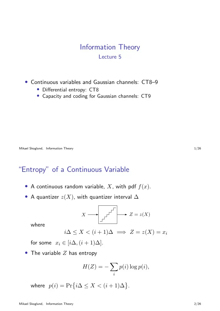
• A continuous random variable, X, with pdf f(x).
• A quantizer z(X), with quantizer interval ∆

X Z = z(X)

where i∆ ≤ X < (i + 1)∆ = ⇒ Z = z(X) = xi for some xi ∈ [i∆, (i + 1)∆].

• The variable Z has entropy

H(Z) = −

• i

p(i) log p(i), where p(i) = Pr

• i∆ ≤ X < (i + 1)∆
• .

Mikael Skoglund, Information Theory 2/26

• Notice that

p(i) = (i+1)∆

i∆

f(x)dx = f(xi)∆ for some xi ∈ [i∆, (i + 1)∆]. Hence for small ∆, we get H(Z) = −

• i

f(xi)∆ log

• f(xi)∆
• = −
• i

f(xi)∆ log f(xi) − log ∆ ≈ − ∞

−∞

f(x) log f(x)dx − log ∆ (if f(x) is Riemann integrable).

Mikael Skoglund, Information Theory 3/26

• Define the differential entropy h(X), or h(f), of X as

h(X) −

• f(x) log f(x)dx

(if the integral exists).

• Then for small ∆

H(Z) + log ∆ ≈ h(X)

• Note that H(Z) → ∞, in general, even if h(X) exists and is finite;
• h(X) is not “entropy,” and H(Z) → h(X) does not hold!

Mikael Skoglund, Information Theory 4/26

• Maximum differential entropy:

For any random variable X with pdf f(x) such that E[X2] =

• x2f(x)dx = P

it holds that h(X) ≤ 1 2 log 2πeP with equality iff f(x) = N(0, P).

Mikael Skoglund, Information Theory 5/26

Typical Sets for Continuous Variables

• A discrete-time continuous-amplitude i.i.d. process {Xm}, with

marginal pdf f(x) of support X.

• It holds that

− lim

n→∞

1 n log f(Xn

1 ) = −E log f(X1) = h(f) a.s.

• Define the typical set A(n)

ε , with respect to f(x), as

A(n)

ε

=

• xn

1 ∈ X n :

• − 1

n log f(xn

1) − h(f)

• ≤ ε
• For A ⊂ Rn, define

Vol(A)

• A

dxn

1

Mikael Skoglund, Information Theory 6/26

• For n sufficiently large

Pr

• Xn

1 ∈ A(n) ε

• =
• A(n)

ε

f(xn

1)dxn 1 > 1 − ε

and Vol

• A(n)

ε

• ≥ (1 − ε)2n(h(f)−ε)
• For all n

Vol

• A(n)

ε

• ≤ 2n(h(f)+ε)
• Since Vol
• A(n)

ε

• ≈ 2nh(f) =
• 2h(f)n, h(f) is the logarithm of the

side-length of a hypercube with the same volume as A(n)

ε .

• Low h(f) =

⇒ Xn

1 typically lives in a small subset of Rn.

• Jointly typical sequences: Straightforward extension.

Mikael Skoglund, Information Theory 7/26

Relative Entropy and Mutual Information

• Define the relative entropy between the pdfs f and g as

D(fg) =

• f(x) log f(x)

g(x) dx and the mutual information between (X, Y ) ∼ f(x, y) as I(X; Y ) = D

• f(x, y)f(x)f(y)
• =
• f(x, y) log f(x, y)

f(x)f(y) dxdy

• While h(X), for a continuous real-valued X, does not have an

interpretation as “entropy,” both D(fg) and I(X; Y ) have equivalent interpretations as in the discrete case.

Mikael Skoglund, Information Theory 8/26

• In fact, both relative entropy and mutual information exist, and their
• perational interpretations stay intact, under very general conditions.
• Let X ∈ X and Y ∈ Y be random variables (or “measurable

functions”) defined on a common abstract probability space (Ω, B, P). Let q(x) and r(y) be “quantizers” that map X and Y , respectively, into real-valued discrete versions q(X) and r(Y ). Then, mutual information is defined as I(X; Y ) sup I

• q(X); r(Y )
• ,
• ver all quantizers q and r. (The two previous definitions of I(X; Y )

are then special cases of this general definition.)

Mikael Skoglund, Information Theory 9/26

The Gaussian Channel

• A continuous-alphabet memoryless channel (X, f(y|x), Y) maps a

continuous real-valued channel input X ∈ X to a continuous real-valued channel output Y ∈ Y, in a stochastic and memoryless manner as described by the conditional pdf f(y|x).

• A memoryless Gaussian channel (with noise variance σ2) is defined as

X = Y = R, and f(y|x) = 1 √ 2πσ2 exp

• −

1 2σ2 (y − x)2 . That is, for a given X = x the channel adds zero mean Gaussian “noise” Z, of variance σ2, such that the variable Y = x + Z is measured at its output.

Mikael Skoglund, Information Theory 10/26

• Coding for a continuous X: if X is very large, or even X = R, coding

needs to be defined subject to a power constraint.

• An (M, n) code with an average power constraint P:

1 An index set IM {1, . . . , M}. 2 An encoder mapping α : IM → X n, which defines the codebook

Cn

• xn

1 : xn 1 = α(i), ∀ i ∈ IM

• =
• xn

1(1), . . . , xn 1(M)

• ,

subject to 1 n

n

• m=1

x2

m(i) ≤ P,

∀ i ∈ IM.

3 A decoder mapping β : Yn → IM.

Mikael Skoglund, Information Theory 11/26

• A rate

R log M n is achievable (subject to the power constraint P) if there exists a sequence of (⌈2nR⌉, n) codes with codewords satisfying the power constraint, and such that the maximal probability of error λ(n) = max

i

Pr

• β(Y n

1 ) = i | Xn 1 = xn 1(i)

• tends to 0 as n → ∞.

The capacity C is the supremum of all rates that are achievable over the channel.

Mikael Skoglund, Information Theory 12/26

Memoryless Gaussian Channel: Lower Bound for C

• Gaussian random code design: Fix the distribution

f(x) = 1

• 2π(P − ε)

exp

• −

x2 2(P − ε)

• and draw

Cn =

• Xn

1 (1), . . . , Xn 1 (M)

• i.i.d. according to

f(xn

1) =

• m

f(xm).

• Encoding: A message ω ∈ IM is encoded as Xn

1 (ω)

Mikael Skoglund, Information Theory 13/26

• Transmission: Received sequence

Y n

1 = Xn 1 (ω) + Zn 1

where {Zm} are i.i.d. zero-mean Gaussian with E[Z2

m] = σ2.

• Decoding: Declare ˆ

ω = β(Y n

1 ) = i if Xn 1 (i) is the only codeword

such that (Xn

1 (i), Y n 1 ) ∈ A(n) ε

and in addition 1

n

n

m=1 X2 m(i) ≤ P, otherwise set ˆ

ω = 0.

• Average probability of error:

πn = Pr

• ˆ

ω = ω

• =
• symmetry
• = Pr
• ˆ

ω = 1 | ω = 1

• with “Pr” over the random codebook and the noise.

Mikael Skoglund, Information Theory 14/26

• Let

E0 = 1 n

• m X2

m(1) > P

• and

Ei =

• Xn

1 (i), Xn 1 (1) + Zn 1

• ∈ A(n)

ε

• then

πn = P(E0 ∪ Ec

1 ∪ E2 ∪ · · · ∪ EM)

≤ P(E0) + P(Ec

1) +

M

i=2 P(Ei)

• Fix a small ε > 0:
• Law of large numbers: P(E0) < ε for sufficiently large n, since

1 n

n

m=1 X2 m(1) → P − ε a.s.

• Joint AEP: P(Ec

1) < ε for sufficiently large n.

• Definition of joint typicality:

P(Ei) ≤ 2−n(I(X;Y )−3ε), i = 2, . . . , M.

Mikael Skoglund, Information Theory 15/26

• For sufficiently large n, we thus get

πn ≤ 2ε + 2−n(I(X;Y )−R−3ε) with I(X; Y ) =

• f(y|x)f(x) log

f(y|x)

• f(y|x)f(x)dxdxdy

where f(x) = N(0, P − ε) generated the codebook and f(y|x) is given by the channel. Since f(y|x) = N(x, σ2) I(X; Y ) = 1 2 log

• 1 + P − ε

σ2

• Mikael Skoglund,

Information Theory 16/26

• As long as R < I(X; Y ) − 3ε, πn → 0 as n → ∞ =

⇒ exists at least

• ne code, say C∗

n, with P n e → 0 for R < I(X; Y ) − 3ε

• Throw away worst half of the codewords in C∗

n to strengthen from

P (n)

e

to λ(n) (the worst half has the codewords that do not satisfy the power constraint, i.e., λi = 1) = ⇒ all R < 1 2 log

• 1 + P − ε

σ2

• are achievable for all ε > 0 =

⇒ C ≥ 1 2 log

• 1 + P

σ2

• Mikael Skoglund,

Information Theory 17/26

Memoryless Gaussian Channel: An Upper Bound for C

• Consider any sequence of codes that can achieve the rate R, that is

λ(n) → 0 and 1

n

n

m=1 x2 m(i) ≤ P, ∀n.

• Assume ω ∈ IM equally likely. Fano =

⇒ R ≤ 1 n

n

• m=1

I(xm(ω); Ym) + ǫn where ǫn = 1

n + RP (n) e

→ 0 as n → ∞, and where I(xm(ω); Ym) = h(Ym) − h(Zm) = h(Ym) − 1 2 log 2πeσ2

Mikael Skoglund, Information Theory 18/26

• Since E[Y 2

m] = Pm + σ2 where Pm = 1 M

M

i=1 x2 m(i) we get

h(Ym) ≤ 1 2 log 2πe(σ2 + Pm) and hence I(xm(ω); Ym) ≤ 1

2 log(1 + Pm σ2 ). Thus,

R ≤ 1 n

n

• m=1

1 2 log

• 1 + Pm

σ2

• + ǫn

≤ 1 2 log

• 1 +

1 n

• m Pm

σ2

• + ǫn

≤ 1 2 log

• 1 + P

σ2

• + ǫn → 1

2 log

• 1 + P

σ2

• as n → ∞

for all achievable R, due to Jensen’s inequality and the power constraint = ⇒ C ≤ 1 2 log

• 1 + P

σ2

• Mikael Skoglund,

Information Theory 19/26

The Coding Theorem for a Memoryless Gaussian Channel

Theorem

A memoryless Gaussian channel with noise variance σ2 and power constraint P has capacity C = 1 2 log

• 1 + P

σ2

• That is, all rates R < C and no rates R > C are achievable.

Mikael Skoglund, Information Theory 20/26

AWGN Capacity vs. Simple Binary Scheme

−4 −2 2 4 6 8 10 12 14 1 2 SNR = 10 · log10

P σ2

bpcs

Capacity 2-PAM

Simple binary scheme:

• Two possible input values: X ∈ {−

√ P, √ P}

• Continuous output (soft decoder): Y = X + Z ∈ R
• Rate: I(X; Y ) = h(X + Z) − h(Z)

Mikael Skoglund, Information Theory 21/26

Parallel Gaussian Channels

• Consider the scenario where there are K available channels

Yk = Xk + Zk, k = 1, . . . K, that can be used simultaneously. Here we assume that Zk are zero-mean independent Gaussian, with E[Z2

k] = σ2 k.

• The capacity of the equivalent “super-channel” is obtained by

signaling independently with powers Pk = E[X2

k] determined as

Pk =

• β − σ2

k,

σ2

k < β

0, σ2

k ≥ β

where β is chosen such that

k Pk = P, the total transmit power.

Mikael Skoglund, Information Theory 22/26

β σ2

1

σ2

2

σ2

3

σ2

4

P1 P2 P3 “water-filling”

• The total capacity is then the sum of the capacities of the individual

sub-channels C = 1 2

K

• k=1

log

• 1 + Pk

σ2

k

• ,

where Pk was defined previously.

• All channels “linearly related” to a set of parallel Gaussian channels

can be handled using the above results!

Mikael Skoglund, Information Theory 23/26

Gaussian Waveform Channel

X(t)

• − T

2 , T 2

• H(f)

+ N(f) Y (t)

• − T

2 , T 2

• Linear-filter waveform channel with Gaussian noise
• Independent Gaussian noise with spectral density N(f)
• Linear filter H(f)
• Input and output confined to time interval
• − T

2 , T 2

• Power constraint

1 T T/2

−T/2

E[X2(t)]dt ≤ P

Mikael Skoglund, Information Theory 24/26

N(f)/|H(f)|2 β S(f) f

• This channel has capacity (in bits per second) given by

C = 1 2

• F(β)

log |H(f)|2 · β N(f) d f P =

• F(β)
• β −

N(f) |H(f)|2

• d

f where F(β) =

• f : N(f) · |H(f)|−2 ≤ β
• and where different possible pairs (C, P) correspond to different

values of β ∈ (0, ∞).

Mikael Skoglund, Information Theory 25/26

• That is, there exists a code (set of M possible input waveforms) such

that arbitrarily low error probability is possible as long as R = log M T < C and as T → ∞. For R > C the error probability is > 0.

• The famous special case of a band-limited AWGN channel:
• Perfect low-pass filter of bandwidth W

H(f) =

• 1

|f| ≤ W |f| > W

• White Gaussian noise, with N(f) = N0/2
• The capacity of this channel is (Shannon ’48):

C = W · log

• 1 +

P WN0

• [bits per second]

Mikael Skoglund, Information Theory 26/26