overview coding and information theory
play

Overview Coding and Information Theory What is information theory? - PowerPoint PPT Presentation

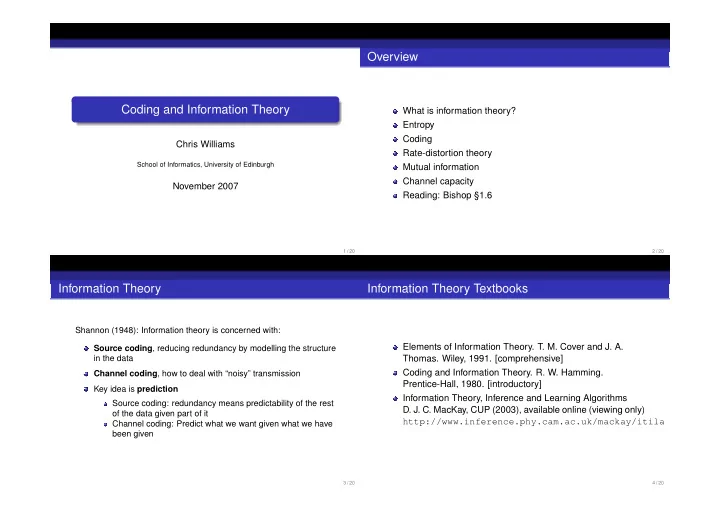
Overview Coding and Information Theory What is information theory? Entropy Coding Chris Williams Rate-distortion theory School of Informatics, University of Edinburgh Mutual information Channel capacity November 2007 Reading: Bishop 1.6


  1. Overview Coding and Information Theory What is information theory? Entropy Coding Chris Williams Rate-distortion theory School of Informatics, University of Edinburgh Mutual information Channel capacity November 2007 Reading: Bishop §1.6 1 / 20 2 / 20 Information Theory Information Theory Textbooks Shannon (1948): Information theory is concerned with: Elements of Information Theory. T. M. Cover and J. A. Source coding , reducing redundancy by modelling the structure in the data Thomas. Wiley, 1991. [comprehensive] Coding and Information Theory. R. W. Hamming. Channel coding , how to deal with “noisy” transmission Prentice-Hall, 1980. [introductory] Key idea is prediction Information Theory, Inference and Learning Algorithms Source coding: redundancy means predictability of the rest D. J. C. MacKay, CUP (2003), available online (viewing only) of the data given part of it http://www.inference.phy.cam.ac.uk/mackay/itila Channel coding: Predict what we want given what we have been given 3 / 20 4 / 20

  2. Entropy Joint entropy, conditional entropy � A discrete random variable X takes on values from an alphabet H ( X , Y ) = − P ( x , y ) log P ( x , y ) X , and has probability mass function P ( x ) = P ( X = x ) for x , y x ∈ X . The entropy H ( X ) of X is defined as � H ( Y | X ) = P ( x ) H ( Y | X = x ) x � H ( X ) = − P ( x ) log P ( x ) � � = − P ( x ) P ( y | x ) log P ( y | x ) x ∈X x y = − E P ( x , y ) log P ( y | x ) convention: for P ( x ) = 0, 0 × log 1 / 0 ≡ 0 H ( X , Y ) = H ( X ) + H ( Y | X ) The entropy measures the information content or “uncertainty” of X . If X , Y are independent Units: log 2 ⇒ bits; log e ⇒ nats. H ( X , Y ) = H ( X ) + H ( Y ) 5 / 20 6 / 20 Coding theory Practical coding methods A coding scheme C assigns a code C ( x ) to every symbol x ; C ( x ) has length ℓ ( x ) . The expected code length L ( C ) of the code is How can we come close to the lower bound ? � L ( C ) = p ( x ) ℓ ( x ) Huffman coding x ∈X Theorem 1: Noiseless coding theorem H ( X ) ≤ L ( C ) < H ( X ) + 1 The expected length L ( C ) of any instantaneous code for X is bounded below by H ( X ) , i.e. Use blocking to reduce the extra bit to an arbitrarily small amount. L ( C ) ≥ H ( X ) Arithmetic coding Theorem 2 There exists an instantaneous code such that H ( X ) ≤ L ( C ) < H ( X ) + 1 7 / 20 8 / 20

  3. Coding with the wrong probabilities Coding real data Say we use the wrong probabilities q i to construct a code. Then So far we have discussed coding sequences if iid random variables. But, for example, the pixels in an image are not � L ( C q ) = − p i log q i iid RVs. So what do we do ? i Consider an image having N pixels, each of which can take But on k grey-level values, as a single RV taking on k N values. p i log p i � > 0 if q i � = p i We would then need to estimate probabilities for all k N q i i different images in order to code a particular image ⇒ properly, which is rather difficult for large k and N . L ( C q ) − H ( X ) > 0 One solution is to chop images into blocks, e.g. 8 × 8 i.e. using the wrong probabilities increases the minimum pixels, and code each block separately. attainable average code length. 9 / 20 10 / 20 Rate-distortion theory • Predictive encoding – try to predict the current pixel value What happens if we can’t afford enough bits to code all of the given nearby context. Successful prediction reduces symbols exactly ? We must be prepared for lossy compression, uncertainty. when two different symbols are assigned the same code. In order to minimize the errors caused by this, we need a distortion function d ( x i , x j ) which measures how much error is caused when symbol x i codes for x j . x x x x H ( X 1 , X 2 ) = H ( X 1 ) + H ( X 2 | X 1 ) The k -means algorithm is a method of choosing code book vectors so as to minimize the expected distortion for d ( x i , x j ) = ( x i − x j ) 2 11 / 20 12 / 20

  4. Source coding Patterns that we observe have a lot of structure, e.g. visual scenes that we care about don’t look like “snow” on the TV Q: Why is coding so important? This gives rise to redundancy , i.e. that observing part of a A: Because of the lossless coding theorem: the best scene will help us predict other parts probabilistic model of the data will have the shortest code This redundancy can be exploited to code the data efficiently— loss less compression Source coding gives us a way of comparing and evaluating different models of data, and searching for good ones Usually we will build models with hidden variables — a new representation of the data 13 / 20 14 / 20 Mutual information Mutual Information I ( X ; Y ) = KL ( p ( x , y ) , p ( x ) p ( y )) ≥ 0 Example 1: p ( x , y ) log p ( x , y ) � Y = p ( x ) p ( y ) = I ( Y ; X ) 1 x , y non p ( x , y ) log p ( x | y ) smoker smoker � = p ( x ) x , y lung = H ( X ) − H ( X | Y ) 1/3 0 cancer = H ( X ) + H ( Y ) − H ( X , Y ) Y 2 no lung Mutual information is a measure of the amount of information 0 2/3 cancer that one RV contains about another. It is the reduction in uncertainty of one RV due to knowledge of the other. Zero mutual information if X and Y are independent 15 / 20 16 / 20

  5. Continuous variables • Example 2: Y 1 non smoker smoker lung 1/9 2/9 cancer Y 2 no lung 2/9 4/9 cancer P ( y 1 ) P ( y 2 ) dy 1 dy 2 = − 1 P ( y 1 , y 2 ) � � 2 log ( 1 − ρ 2 ) I ( Y 1 ; Y 2 ) = P ( y 1 , y 2 ) log 17 / 20 18 / 20 PCA and mutual information Channel capacity Linsker, 1988, Principle of maximum information preservation Consider a random variable Y = a T X + ǫ , with a T a = 1. The channel capacity of a discrete memoryless channel is How do we maximize I ( Y ; X ) ? defined as C = max p ( x ) I ( X ; Y ) I ( Y ; X ) = H ( Y ) − H ( Y | X ) Noisy channel coding theorem But H ( Y | X ) is just the entropy of the noise term ǫ . If X has a (Informal statement) Error free communication above the joint multivariate Gaussian distribution then Y will have a channel capacity is impossible; communication at bit rates Gaussian distribution. The (differential) entropy of a Gaussian below C is possible with arbitrarily small error. N ( µ, σ 2 ) is 1 2 log 2 π e σ 2 . Hence we maximize information preservation by choosing a to give Y maximum variance subject to the constraint a T a = 1. 19 / 20 20 / 20

Download Presentation
Download Policy: The content available on the website is offered to you 'AS IS' for your personal information and use only. It cannot be commercialized, licensed, or distributed on other websites without prior consent from the author. To download a presentation, simply click this link. If you encounter any difficulties during the download process, it's possible that the publisher has removed the file from their server.

Recommend


More recommend