Inference by enumeration Slightly intelligent way to sum out - PDF document

Inference by enumeration Slightly intelligent way to sum out variables from the joint without actually constructing its explicit representation Simple query on the burglary network: Inference in Bayesian networks B E P ( B | j, m ) = P ( B, j, m ) /P ( j, m ) A = α P ( B, j, m ) J M = α Σ e Σ a P ( B, e, a, j, m ) Chapter 14.4–5 Rewrite full joint entries using product of CPT entries: P ( B | j, m ) = α Σ e Σ a P ( B ) P ( e ) P ( a | B, e ) P ( j | a ) P ( m | a ) = α P ( B ) Σ e P ( e ) Σ a P ( a | B, e ) P ( j | a ) P ( m | a ) Recursive depth-first enumeration: O ( n ) space, O ( d n ) time Chapter 14.4–5 1 Chapter 14.4–5 4 Outline Enumeration algorithm ♦ Exact inference by enumeration function Enumeration-Ask ( X , e , bn ) returns a distribution over X inputs : X , the query variable ♦ Approximate inference by stochastic simulation e , observed values for variables E bn , a Bayesian network with variables { X } ∪ E ∪ Y Q ( X ) ← a distribution over X , initially empty for each value x i of X do extend e with value x i for X Q ( x i ) ← Enumerate-All ( Vars [ bn ], e ) return Normalize ( Q ( X ) ) function Enumerate-All ( vars , e ) returns a real number if Empty? 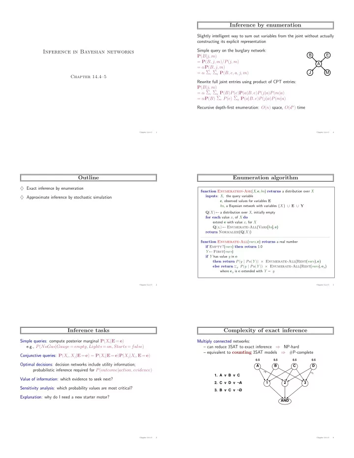( vars ) then return 1.0 Y ← First ( vars ) if Y has value y in e then return P ( y | Pa ( Y )) × Enumerate-All ( Rest ( vars ), e ) else return y P ( y | Pa ( Y )) × Enumerate-All ( Rest ( vars ), e y ) � where e y is e extended with Y = y Chapter 14.4–5 2 Chapter 14.4–5 5 Inference tasks Complexity of exact inference Simple queries: compute posterior marginal P ( X i | E = e ) Multiply connected networks: e.g., P ( NoGas | Gauge = empty, Lights = on, Starts = false ) – can reduce 3SAT to exact inference ⇒ NP-hard – equivalent to counting 3SAT models ⇒ #P-complete Conjunctive queries: P ( X i , X j | E = e ) = P ( X i | E = e ) P ( X j | X i , E = e ) 0.5 0.5 0.5 0.5 Optimal decisions: decision networks include utility information; A B C D probabilistic inference required for P ( outcome | action, evidence ) L 1. A v B v C L Value of information: which evidence to seek next? 2. C v D v A 1 2 3 L Sensitivity analysis: which probability values are most critical? 3. B v C v D L Explanation: why do I need a new starter motor? AND Chapter 14.4–5 3 Chapter 14.4–5 6

Inference by stochastic simulation Example P(C) Basic idea: .50 1) Draw N samples from a sampling distribution S 0.5 2) Compute an approximate posterior probability ˆ P Cloudy 3) Show this converges to the true probability P Coin Outline: C P(S|C) C P(R|C) – Sampling from an empty network Rain T .10 Sprinkler T .80 – Rejection sampling: reject samples disagreeing with evidence F .50 F .20 – Likelihood weighting: use evidence to weight samples Wet Grass S R P(W|S,R) T T .99 T F .90 F T .90 F F .01 Chapter 14.4–5 7 Chapter 14.4–5 10 Sampling from an empty network Example P(C) function Prior-Sample ( bn ) returns an event sampled from bn .50 inputs : bn , a belief network specifying joint distribution P ( X 1 , . . . , X n ) Cloudy x ← an event with n elements for i = 1 to n do x i ← a random sample from P ( X i | parents ( X i )) C P(S|C) C P(R|C) given the values of Parents ( X i ) in x Rain T .10 Sprinkler T .80 return x F .50 F .20 Wet Grass S R P(W|S,R) T T .99 T F .90 F T .90 F F .01 Chapter 14.4–5 8 Chapter 14.4–5 11 Example Example P(C) P(C) .50 .50 Cloudy Cloudy C P(S|C) C P(R|C) C P(S|C) C P(R|C) Rain Rain T .10 Sprinkler T .80 T .10 Sprinkler T .80 F .50 F .20 F .50 F .20 Wet Wet Grass Grass S R P(W|S,R) S R P(W|S,R) T T .99 T T .99 T F .90 T F .90 F T .90 F T .90 F F .01 F F .01 Chapter 14.4–5 9 Chapter 14.4–5 12

Example Sampling from an empty network contd. P(C) Probability that PriorSample generates a particular event .50 S PS ( x 1 . . . x n ) = Π n i = 1 P ( x i | parents ( X i )) = P ( x 1 . . . x n ) i.e., the true prior probability Cloudy E.g., S PS ( t, f, t, t ) = 0 . 5 × 0 . 9 × 0 . 8 × 0 . 9 = 0 . 324 = P ( t, f, t, t ) C P(S|C) C P(R|C) Let N PS ( x 1 . . . x n ) be the number of samples generated for event x 1 , . . . , x n Rain T .10 Sprinkler T .80 Then we have F .50 F .20 ˆ Wet lim P ( x 1 , . . . , x n ) = N →∞ N PS ( x 1 , . . . , x n ) /N lim Grass N →∞ = S PS ( x 1 , . . . , x n ) S R P(W|S,R) = P ( x 1 . . . x n ) T T .99 That is, estimates derived from PriorSample are consistent T F .90 F T .90 Shorthand: ˆ P ( x 1 , . . . , x n ) ≈ P ( x 1 . . . x n ) F F .01 Chapter 14.4–5 13 Chapter 14.4–5 16 Example Rejection sampling P(C) ˆ P ( X | e ) estimated from samples agreeing with e .50 function Rejection-Sampling ( X , e , bn , N ) returns an estimate of P ( X | e ) Cloudy local variables : N , a vector of counts over X , initially zero for j = 1 to N do C P(S|C) C P(R|C) x ← Prior-Sample ( bn ) Rain T .10 Sprinkler T .80 if x is consistent with e then N [ x ] ← N [ x ]+1 where x is the value of X in x F .50 F .20 return Normalize ( N [ X ]) Wet Grass E.g., estimate P ( Rain | Sprinkler = true ) using 100 samples S R P(W|S,R) 27 samples have Sprinkler = true T T .99 Of these, 8 have Rain = true and 19 have Rain = false . T F .90 ˆ P ( Rain | Sprinkler = true ) = Normalize ( � 8 , 19 � ) = � 0 . 296 , 0 . 704 � F T .90 F F .01 Similar to a basic real-world empirical estimation procedure Chapter 14.4–5 14 Chapter 14.4–5 17 Example Analysis of rejection sampling P(C) ˆ P ( X | e ) = α N PS ( X, e ) (algorithm defn.) .50 = N PS ( X, e ) /N PS ( e ) (normalized by N PS ( e ) ) ≈ P ( X, e ) /P ( e ) (property of PriorSample ) Cloudy = P ( X | e ) (defn. of conditional probability) C P(S|C) C P(R|C) Hence rejection sampling returns consistent posterior estimates Rain T .10 Sprinkler T .80 Problem: hopelessly expensive if P ( e ) is small F .50 F .20 P ( e ) drops off exponentially with number of evidence variables! Wet Grass S R P(W|S,R) T T .99 T F .90 F T .90 F F .01 Chapter 14.4–5 15 Chapter 14.4–5 18

Likelihood weighting Likelihood weighting example P(C) Idea: fix evidence variables, sample only nonevidence variables, .50 and weight each sample by the likelihood it accords the evidence Cloudy function Likelihood-Weighting ( X , e , bn , N ) returns an estimate of P ( X | e ) local variables : W , a vector of weighted counts over X , initially zero C P(S|C) C P(R|C) Rain T .10 Sprinkler T .80 for j = 1 to N do F .50 F .20 x , w ← Weighted-Sample ( bn ) W [ x ] ← W [ x ] + w where x is the value of X in x Wet Grass return Normalize ( W [ X ] ) S R P(W|S,R) function Weighted-Sample ( bn , e ) returns an event and a weight T T .99 T F .90 x ← an event with n elements; w ← 1 F T .90 for i = 1 to n do F F .01 if X i has a value x i in e then w ← w × P ( X i = x i | parents ( X i )) else x i ← a random sample from P ( X i | parents ( X i )) w = 1 . 0 return x , w Chapter 14.4–5 19 Chapter 14.4–5 22 Likelihood weighting example Likelihood weighting example P(C) P(C) .50 .50 Cloudy Cloudy C P(S|C) C P(R|C) C P(S|C) C P(R|C) Rain Rain T .10 Sprinkler T .80 T .10 Sprinkler T .80 F .50 F .20 F .50 F .20 Wet Wet Grass Grass S R P(W|S,R) S R P(W|S,R) T T .99 T T .99 T F .90 T F .90 F T .90 F T .90 F F .01 F F .01 w = 1 . 0 w = 1 . 0 × 0 . 1 Chapter 14.4–5 20 Chapter 14.4–5 23 Likelihood weighting example Likelihood weighting example P(C) P(C) .50 .50 Cloudy Cloudy C P(S|C) C P(R|C) C P(S|C) C P(R|C) Rain Rain T .10 Sprinkler T .80 T .10 Sprinkler T .80 F .50 F .20 F .50 F .20 Wet Wet Grass Grass S R P(W|S,R) S R P(W|S,R) T T .99 T T .99 T F .90 T F .90 F T .90 F T .90 F F .01 F F .01 w = 1 . 0 w = 1 . 0 × 0 . 1 Chapter 14.4–5 21 Chapter 14.4–5 24

Likelihood weighting example Summary P(C) Exact inference by enumeration: .50 – NP-hard on general graphs Cloudy Approximate inference by LW: – LW does poorly when there is lots of (downstream) evidence C P(S|C) C P(R|C) – LW, generally insensitive to topology Rain T .10 Sprinkler T .80 F .50 F .20 – Convergence can be very slow with probabilities close to 1 or 0 – Can handle arbitrary combinations of discrete and continuous variables Wet Grass S R P(W|S,R) T T .99 T F .90 F T .90 F F .01 w = 1 . 0 × 0 . 1 Chapter 14.4–5 25 Chapter 14.4–5 28 Likelihood weighting example P(C) .50 Cloudy C P(S|C) C P(R|C) Rain T .10 Sprinkler T .80 F .50 F .20 Wet Grass S R P(W|S,R) T T .99 T F .90 F T .90 F F .01 w = 1 . 0 × 0 . 1 × 0 . 99 = 0 . 099 Chapter 14.4–5 26 Likelihood weighting analysis Sampling probability for WeightedSample is S WS ( z , e ) = Π l i = 1 P ( z i | parents ( Z i )) Note: pays attention to evidence in ancestors only Cloudy ⇒ somewhere “in between” prior and posterior distribution Sprinkler Rain Wet Weight for a given sample z , e is Grass w ( z , e ) = Π m i = 1 P ( e i | parents ( E i )) Weighted sampling probability is S WS ( z , e ) w ( z , e ) = Π l i = 1 P ( z i | parents ( Z i )) Π m i = 1 P ( e i | parents ( E i )) = P ( z , e ) (by standard global semantics of network) Hence likelihood weighting returns consistent estimates but performance still degrades with many evidence variables because a few samples have nearly all the total weight Chapter 14.4–5 27