Example Topology of network encodes conditional independence - - PDF document

Bayesian networks

Chapter 14.1–3

Outline

♦ Syntax ♦ Semantics ♦ Parameterized distributions

Bayesian networks

A simple, graphical notation for conditional independence assertions and hence for compact specification of full joint distributions Syntax: a set of nodes, one per variable a directed, acyclic graph (link ≈ “directly influences”) a conditional distribution for each node given its parents: P(Xi|Parents(Xi)) In the simplest case, conditional distribution represented as a conditional probability table (CPT) giving the distribution over Xi for each combination of parent values

Example

Topology of network encodes conditional independence assertions: Weather Cavity Toothache Catch Weather is independent of the other variables Toothache and Catch are conditionally independent given Cavity

Example

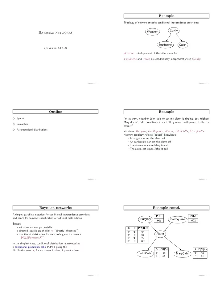
I’m at work, neighbor John calls to say my alarm is ringing, but neighbor Mary doesn’t call. Sometimes it’s set off by minor earthquakes. Is there a burglar? Variables: Burglar, Earthquake, Alarm, JohnCalls, MaryCalls Network topology reflects “causal” knowledge: – A burglar can set the alarm off – An earthquake can set the alarm off – The alarm can cause Mary to call – The alarm can cause John to call

Example contd.

.001

P(B)

.002

P(E)

Alarm Earthquake MaryCalls JohnCalls Burglary

B

T T F F

E

T F T F .95 .29 .001 .94

P(A|B,E) A

T F .90 .05

P(J|A) A

T F .70 .01

P(M|A)

Compactness

A CPT for Boolean Xi with k Boolean parents has

B E J A M

2k rows for the combinations of parent values Each row requires one number p for Xi = true (the number for Xi = false is just 1 − p) If each variable has no more than k parents, the complete network requires O(n · 2k) numbers I.e., grows linearly with n, vs. O(2n) for the full joint distribution For burglary net, ?? numbers

Compactness

A CPT for Boolean Xi with k Boolean parents has

B E J A M

2k rows for the combinations of parent values Each row requires one number p for Xi = true (the number for Xi = false is just 1 − p) If each variable has no more than k parents, the complete network requires O(n · 2k) numbers I.e., grows linearly with n, vs. O(2n) for the full joint distribution For burglary net, 1 + 1 + 4 + 2 + 2 = 10 numbers (vs. 25 − 1 = 31)

Global semantics

Global semantics defines the full joint distribution

B E J A M

as the product of the local conditional distributions: P(x1, . . . , xn) = Πn

i = 1P(xi|parents(Xi))

e.g., P(j ∧ m ∧ a ∧ ¬b ∧ ¬e) =

Global semantics

“Global” semantics defines the full joint distribution

B E J A M

as the product of the local conditional distributions: P(x1, . . . , xn) = Πn

i = 1P(xi|parents(Xi))

e.g., P(j ∧ m ∧ a ∧ ¬b ∧ ¬e) = P(j|a)P(m|a)P(a|¬b, ¬e)P(¬b)P(¬e) = 0.9 × 0.7 × 0.001 × 0.999 × 0.998 ≈ 0.00063

Constructing Bayesian networks

Need a method such that a series of locally testable assertions of conditional independence guarantees the required global semantics

• 1. Choose an ordering of variables X1, . . . , Xn
• 2. For i = 1 to n

add Xi to the network select parents from X1, . . . , Xi−1 such that P(Xi|Parents(Xi)) = P(Xi|X1, . . . , Xi−1)

Constructing Bayesian networks

Need a method such that a series of locally testable assertions of conditional independence guarantees the required global semantics

• 1. Choose an ordering of variables X1, . . . , Xn
• 2. For i = 1 to n

add Xi to the network select parents from X1, . . . , Xi−1 such that P(Xi|Parents(Xi)) = P(Xi|X1, . . . , Xi−1) This choice of parents guarantees the global semantics: P(X1, . . . , Xn) = Πn

i = 1P(Xi|X1, . . . , Xi−1)

(chain rule) = Πn

i = 1P(Xi|Parents(Xi))

(by construction)

Example

Suppose we choose the ordering M, J, A, B, E

MaryCalls JohnCalls

P(J|M) = P(J)?

Example

Suppose we choose the ordering M, J, A, B, E

MaryCalls Alarm JohnCalls

P(J|M) = P(J)? No P(A|J, M) = P(A|J)? P(A|J, M) = P(A)?

Example

Suppose we choose the ordering M, J, A, B, E

MaryCalls Alarm Burglary JohnCalls

P(J|M) = P(J)? No P(A|J, M) = P(A|J)? P(A|J, M) = P(A)? No P(B|A, J, M) = P(B|A)? P(B|A, J, M) = P(B)?

Example

Suppose we choose the ordering M, J, A, B, E

MaryCalls Alarm Burglary Earthquake JohnCalls

P(J|M) = P(J)? No P(A|J, M) = P(A|J)? P(A|J, M) = P(A)? No P(B|A, J, M) = P(B|A)? Yes P(B|A, J, M) = P(B)? No P(E|B, A, J, M) = P(E|A)? P(E|B, A, J, M) = P(E|A, B)?

Example

Suppose we choose the ordering M, J, A, B, E

MaryCalls Alarm Burglary Earthquake JohnCalls

P(J|M) = P(J)? No P(A|J, M) = P(A|J)? P(A|J, M) = P(A)? No P(B|A, J, M) = P(B|A)? Yes P(B|A, J, M) = P(B)? No P(E|B, A, J, M) = P(E|A)? No P(E|B, A, J, M) = P(E|A, B)? Yes

Example contd.

MaryCalls Alarm Burglary Earthquake JohnCalls

Deciding conditional independence is hard in noncausal directions (Causal models and conditional independence seem hardwired for humans!) Assessing conditional probabilities is hard in noncausal directions Network is less compact: 1 + 2 + 4 + 2 + 4 = 13 numbers needed

Example: Car diagnosis

Initial evidence: car won’t start Testable variables (green), “broken, so fix it” variables (orange) Hidden variables (gray) ensure sparse structure, reduce parameters

lights no oil no gas starter broken battery age alternator broken fanbelt broken battery dead no charging battery flat gas gauge fuel line blocked

• il light

battery meter car won’t start dipstick

Example: Car insurance

SocioEcon Age GoodStudent ExtraCar Mileage VehicleYear RiskAversion SeniorTrain DrivingSkill MakeModel DrivingHist DrivQuality Antilock Airbag CarValue HomeBase AntiTheft Theft OwnDamage PropertyCost LiabilityCost MedicalCost Cushioning Ruggedness Accident OtherCost OwnCost

Compact conditional distributions

CPT grows exponentially with number of parents CPT becomes infinite with continuous-valued parent or child Solution: canonical distributions that are defined compactly Deterministic nodes are the simplest case: X = f(Parents(X)) for some function f E.g., Boolean functions NorthAmerican ⇔ Canadian ∨ US ∨ Mexican E.g., numerical relationships among continuous variables ∂Level ∂t = inflow + precipitation - outflow - evaporation

Compact conditional distributions contd.

Noisy-OR distributions model multiple noninteracting causes 1) Parents U1 . . . Uk include all causes (can add leak node) 2) Independent failure probability qi for each cause alone ⇒ P(X|U1 . . . Uj, ¬Uj+1 . . . ¬Uk) = 1 − Πj

i = 1qi

Cold Flu Malaria P(Fever) P(¬Fever) F F F 0.0 1.0 F F T 0.9 0.1 F T F 0.8 0.2 F T T 0.98 0.02 = 0.2 × 0.1 T F F 0.4 0.6 T F T 0.94 0.06 = 0.6 × 0.1 T T F 0.88 0.12 = 0.6 × 0.2 T T T 0.988 0.012 = 0.6 × 0.2 × 0.1 Number of parameters linear in number of parents

Hybrid (discrete+continuous) networks

Discrete (Subsidy? and Buys?); continuous (Harvest and Cost)

Buys? Harvest Subsidy? Cost

Option 1: discretization—possibly large errors, large CPTs Option 2: finitely parameterized canonical families 1) Continuous variable, discrete+continuous parents (e.g., Cost) 2) Discrete variable, continuous parents (e.g., Buys?)

Continuous variables

Gaussian density P(x) =

1 √ 2πσe−(x−µ)2/2σ2

Uniform density P(X = x) = U[18, 26](x) = uniform density between 18 and 26

0.125 dx 18 26

Continuous child variables

Need one conditional density function for child variable given continuous parents, for each possible assignment to discrete parents Most common is the linear Gaussian model, e.g.,: P(Cost = c|Harvest = h, Subsidy? = true) = N(ath + bt, σt)(c) = 1 σt √ 2πexp

2

σt

2

Mean Cost varies linearly with Harvest, variance is fixed Linear variation is unreasonable over the full range but works OK if the likely range of Harvest is narrow

Continuous child variables

All-continuous network with LG distributions ⇒ full joint distribution is a multivariate Gaussian Discrete+continuous LG network is a conditional Gaussian network i.e., a multivariate Gaussian over all continuous variables for each combination of discrete variable values

Discrete variable w/ continuous parents

Probability of Buys? given Cost should be a “soft” threshold:

0.2 0.4 0.6 0.8 1 2 4 6 8 10 12 P(Buys?=false|Cost=c) Cost c

Probit distribution uses integral of Gaussian: Φ(x) =

−∞ N(0, 1)(x)dx

P(Buys? = true | Cost = c) = Φ((−c + µ)/σ)

Why the probit?

• 1. It’s sort of the right shape
• 2. Can view as hard threshold whose location is subject to noise

Buys? Cost Cost Noise

Discrete variable contd.

Sigmoid (or logit) distribution also used in neural networks: P(Buys? = true | Cost = c) = 1 1 + exp(−2−c+µ

σ )

Sigmoid has similar shape to probit but much longer tails:

0.1 0.2 0.3 0.4 0.5 0.6 0.7 0.8 0.9 1 2 4 6 8 10 12 P(Buys?=false|Cost=c) Cost c

Summary

Bayes nets provide a natural representation for (causally induced) conditional independence Topology + CPTs = compact representation of joint distribution Generally easy for (non)experts to construct Canonical distributions (e.g., noisy-OR) = compact representation of CPTs Continuous variables ⇒ parameterized distributions (e.g., linear Gaussian)