Coherence Analysis Overview Definition Coherency Definition R xy - - PowerPoint PPT Presentation

coherence analysis overview definition coherency
SMART_READER_LITE
LIVE PREVIEW

Coherence Analysis Overview Definition Coherency Definition R xy - - PowerPoint PPT Presentation

Coherence Analysis Overview Definition Coherency Definition R xy (e j ) Properties G xy ( ) R x (e j ) R y (e j ) Estimation Correlation of complex-valued RVs Also known as the coherency spectrum (Weiner, 1930) or


slide-1
SLIDE 1

What is it Really? G2

xy(ω)

|Rxy(ejω)|2 Rx(ejω)Ry(ejω)

  • Coherence is a measure of correlation in frequency
  • Usual assumptions apply (WSS)
  • For estimation, we require ergodicity
  • J. McNames

Portland State University ECE 538/638 Coherence Analysis

  • Ver. 1.01

3

Coherence Analysis Overview

  • Definition
  • Properties
  • Estimation
  • Correlation of complex-valued RVs
  • Examples
  • Discussion
  • J. McNames

Portland State University ECE 538/638 Coherence Analysis

  • Ver. 1.01

1

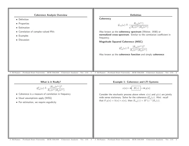
Example 1: Coherence and LTI Systems x(n) y(n) H(z) Consider the stochastic process above where x(n) and y(n) are jointly wide sense stationary. Solve for the coherence G2

xy(ω). Hint: recall

that if y(n) = h(n) ∗ x(n), then Rxy(z) = H∗(z−∗)Rx(z).

  • J. McNames

Portland State University ECE 538/638 Coherence Analysis

  • Ver. 1.01

4

Definition Coherency Gxy(ω) Rxy(ejω)

  • Rx(ejω)Ry(ejω)

Also known as the coherency spectrum (Weiner, 1930) or normalized cross-spectrum. Similar to the correlation coefficient in frequency. Magnitude Squared Coherence (MSC) G2

xy(ω)

|Rxy(ejω)|2 Rx(ejω)Ry(ejω) Also known as the coherence function and simply coherence

  • J. McNames

Portland State University ECE 538/638 Coherence Analysis

  • Ver. 1.01

2

slide-2
SLIDE 2

Example 2: Workspace

  • J. McNames

Portland State University ECE 538/638 Coherence Analysis

  • Ver. 1.01

7

Example 1: Workspace

  • J. McNames

Portland State University ECE 538/638 Coherence Analysis

  • Ver. 1.01

5

Properties G2

xy(ω)

|Rxy(ejω)|2 Rx(ejω)Ry(ejω) Coherence has many interesting and useful properties

  • If y(n) = h(n) ∗ x(n), then G2

xy(ω) = 1

  • If rxy(ℓ) = 0, then
  • G2

xy(ω) = 0 if

– rxy(ℓ) = 0 – x(n) and y(n) are statistically independent

  • Bounded: 0 ≤ G2

xy ≤ 1

  • Symmetry: G2

xy(ω) = G2 yx(ω)

  • Can be applied to complex signals, though range must span

−π < ω < π in that case

  • J. McNames

Portland State University ECE 538/638 Coherence Analysis

  • Ver. 1.01

8

Example 2: Coherence and LTI Systems w(n) x(n) y(n) G(z) H(z) F(z) Σ Consider the stochastic process above where w(n) and x(n) are jointly wide sense stationary and uncorrelated and the LTI systems are all

  • stable. Solve for the coherence G2

xy(ω).

  • J. McNames

Portland State University ECE 538/638 Coherence Analysis

  • Ver. 1.01

6

slide-3
SLIDE 3

Understanding Complex Correlation ρ = E[xy∗]

  • E[xx∗] E[yy∗]

E[xy∗] = E[axejθxaye−jθy] = E[axayej(θx−θy)] E[xx∗] = E[a2

x]

  • ρ will be zero if (θx − θy) ∼ U[0, 2π]
  • If ax and ay are constants, ρ is the phase correlation:

ρ = E[ej(θx−θy)]

  • If (θx − θy) is a constant, |ρ| is the un-normalized correlation

coefficient of the amplitudes ρ = E[axa∗

y]

  • E[a2

x] E[a2 y]

ej(θx−θy)

  • In general is a mixture of phase and amplitude correlation
  • J. McNames

Portland State University ECE 538/638 Coherence Analysis

  • Ver. 1.01

11

Coherence as Correlation G2

xy(ω) =

|Rxy(ejω)|2 Rx(ejω)Ry(ejω) ρ2 = | cov[x, y]|2 var[x] var[y]

  • Coherence is very similar to the coefficient of determination

(square of the correlation coefficient) between two RVs

  • It is, actually, the coherence between the random spectra

x(n) = 1 2π π

−π

ejωndX(ejω) E

  • dX(ejω)
  • 2

= Rx(ejω)dω G2

xy(ω) =

  • cov
  • dX(ejω), dY ∗(ejω)
  • 2

var [dX(ejω)] var [dY (ejω)] but this requires stochastic integrals, which are beyond the scope

  • f this class (see [1, chapter 4])
  • It is therefore worthwhile to understand the difference between

correlation of real- and complex-valued RVs

  • J. McNames

Portland State University ECE 538/638 Coherence Analysis

  • Ver. 1.01

9

Understanding Complex Correlation ρ = E[xy∗]

  • E[xx∗] E[yy∗]

E[xy∗] = E[axejθxaye−jθy] = E[axayej(θx−θy)] E[xx∗] = E[a2

x]

  • Strong correlation, say ρ = 0.90, does not mean could accurately

estimate x from y or vice versa – Sufficient accuracy depends on the application – Also does not mean a linear estimate is best – Could possibly estimate more accurately with nonlinear estimate

  • Weak correlation, say ρ = 0.10, does not mean x and y are

unrelated

  • Only measures degree of linear association of x and y
  • J. McNames

Portland State University ECE 538/638 Coherence Analysis

  • Ver. 1.01

12

Complex Correlation Let x and y be complex-valued zero-mean random variables. The complex correlation coefficient is then defined as ρ = cov[x, y]

  • var[x] var[y]

= E[xy∗]

  • E[xx∗] E[yy∗]
  • ρ will be complex-valued

– Less intuitive than for real-valued variables – Does not retain the sign to indicate positive or negative correlation

  • Can’t look at scatter plot (x, y span four dimensions)
  • J. McNames

Portland State University ECE 538/638 Coherence Analysis

  • Ver. 1.01

10

slide-4
SLIDE 4

Example 3: Complex Correlation Scatter Plots

−1 1 −0.5 0.5 Real(y) N:500 True Correlation:0.900 Real(x) −1 1 −0.5 0.5 Real(y) Estimated Correlation:0.895 Imag(x) −1 1 −0.5 0.5 Imag(y) Real(x) −1 1 −0.5 0.5 Imag(y) Imag(x)

  • J. McNames

Portland State University ECE 538/638 Coherence Analysis

  • Ver. 1.01

15

Understanding Complex Correlation Continued R˜

y(ejω) = Ry(ejω)

  • 1 − G2

xy(ω)

y(ejω) = Ry(ejω)G2 xy(ω)

Ry(ejω) = Rˆ

y(ejω) + R˜ y(ω)

  • Let x(n) and y(n) be zero-mean jointly WSS random processes

– ˆ y(n) = h(n) ∗ x(n) be the best linear estimate of y(n) given x(n) – ˜ y(n) = y(n) − ˆ y(n)

  • Then G2

xy(ω) can be interpreted as the fraction of the variance

explained by an optimal linear model

  • Alternatively the MSC is the fraction of Ry(ejω) that can be

estimated from x(n)

  • J. McNames

Portland State University ECE 538/638 Coherence Analysis

  • Ver. 1.01

13

Example 3: Complex Correlation Ratio Scatter Plot

−6 −4 −2 2 4 6 −4 −3 −2 −1 1 2 3 4 Real Ratio y/x N:500 True Correlation:0.900 Estimated Correlation:0.895 Imaginary

  • J. McNames

Portland State University ECE 538/638 Coherence Analysis

  • Ver. 1.01

16

Example 3: Complex Correlation Scatter Plots Create 500 pairs of IID, zero-mean, unit-variance complex-valued Gaussian RVs, x and y, with a true correlation of ρ = 0.9 and ρ = 0.1. Estimate the absolute value of the correlation coefficient. Plot scatter plots of the real and imaginary components of x and y. Also create a scatter plot of the ratio of x/y. Discuss the results.

  • J. McNames

Portland State University ECE 538/638 Coherence Analysis

  • Ver. 1.01

14

slide-5
SLIDE 5

Example 3: MATLAB Code

N = 500; rho = 0.90; % Desired correlation am = sqrt(rho^2/(1-rho^2)); a = am*exp(-j*pi/4); x = 1/sqrt(2)*(randn(N,1) + j*randn(N,1)); w = 1/sqrt(2)*(randn(N,1) + j*randn(N,1)); y = (w + a*x)./sqrt(1+abs(a)^2); yc = conj(y); xc = conj(x); cyx = sum(y.*xc); cyx2 = cyx * conj(cyx); sxx2 = sum(x.*xc); syy2 = sum(y.*yc); Cyx = sqrt(cyx2/(sxx2*syy2)); % Estimated correlation coefficient

  • J. McNames

Portland State University ECE 538/638 Coherence Analysis

  • Ver. 1.01

19

Example 3: Complex Correlation Scatter Plots

−1 1 −1 1 Real(y) N:500 True Correlation:0.100 Real(x) −1 1 −1 1 Real(y) Estimated Correlation:0.042 Imag(x) −1 1 −1 −0.5 0.5 1 Imag(y) Real(x) −1 1 −1 −0.5 0.5 1 Imag(y) Imag(x)

  • J. McNames

Portland State University ECE 538/638 Coherence Analysis

  • Ver. 1.01

17

Estimation Let x(n) be a WSS process

  • It seems that most people use Welch’s nonparametric PSD and

CPSD estimates (why?)

  • Most of the statistical properties are apparently only known for

Bartlett’s estimate

  • Usual (unrealistic) assumptions apply

– Independent segments – Gaussian process – No spectral leakage

  • J. McNames

Portland State University ECE 538/638 Coherence Analysis

  • Ver. 1.01

20

Example 3: Complex Correlation Ratio Scatter Plot

−6 −4 −2 2 4 6 −4 −3 −2 −1 1 2 3 4 Real Ratio y/x N:500 True Correlation:0.100 Estimated Correlation:0.042 Imaginary

  • J. McNames

Portland State University ECE 538/638 Coherence Analysis

  • Ver. 1.01

18

slide-6
SLIDE 6

Example 4: White Noise Coherence

0.05 0.1 0.15 0.2 0.25 0.3 0.35 0.4 0.45 0.5 0.1 0.2 0.3 0.4 0.5 Frequency (normalized) N:1000 Window:200 |ρ|2:0.250 Estimated |ρ|2:0.267 Estimated Coherence True Coherence

  • J. McNames

Portland State University ECE 538/638 Coherence Analysis

  • Ver. 1.01

23

Signal Plus Noise Example Let x(n) and w(n) be zero-mean WGN processes with variance σ2. y(n) = x(n) + 1

aw(n)

G2(ω) = Rx(ejω) Rx(ejω) + 1

a2 Rw(ejω)

= a2σ2

x

a2σ2

x + σ2 w

= a2 a2 + 1

  • Since all signals are WGN, the PSDs are constant and spectral

leakage does not cause any bias

  • J. McNames

Portland State University ECE 538/638 Coherence Analysis

  • Ver. 1.01

21

Example 4: White Noise Coherence

0.05 0.1 0.15 0.2 0.25 0.3 0.35 0.4 0.45 0.5 0.1 0.2 0.3 0.4 0.5 Frequency (normalized) N:2000 Window:200 |ρ|2:0.250 Estimated |ρ|2:0.226 Estimated Coherence True Coherence

  • J. McNames

Portland State University ECE 538/638 Coherence Analysis

  • Ver. 1.01

24

Example 4: White Noise Coherene Create a single realization of N =1000, 2000, 5000, and 10,000 samples of the random process y(n) = x(n) + 1

aw(n) where x(n) and

w(n) be zero-mean WGN processes with variance σ2. Plot the true and estimated coherence for a window length of 200 samples. What impact does increasing N have on K. What is the effect on ˆ G2

xy(ω)?

  • J. McNames

Portland State University ECE 538/638 Coherence Analysis

  • Ver. 1.01

22

slide-7
SLIDE 7

Sampling Distribution f(|ˆ ρ|2; K, |ρ|2) = (K−1)(1−|ρ|2)K(1−|ˆ ρ|2)K−2

2F1(K, K; 1; |ρ|2|ˆ

ρ|2) for 0 ≤ |ρ|2|ˆ ρ|2 < 1

  • When x and y are K samples of an IID, zero-mean Gaussian RVs,

the distribution of |ˆ ρ|2 is known

  • This same pdf is usually used for G2

xy(ω)

  • Resulting pdf is only approximate for MSC because these

assumptions don’t hold for G2

xy(ω)

– Segments are not independent, even with Bartlett’s method – Spectral leakage

  • 2F1(K, K; 1; |ρ|2|ˆ

ρ|2) is a hypergeometric function (see hypergeom in MATLAB)

  • J. McNames

Portland State University ECE 538/638 Coherence Analysis

  • Ver. 1.01

27

Example 4: White Noise Coherence

0.05 0.1 0.15 0.2 0.25 0.3 0.35 0.4 0.45 0.5 0.1 0.2 0.3 0.4 0.5 Frequency (normalized) N:5000 Window:200 |ρ|2:0.250 Estimated |ρ|2:0.254 Estimated Coherence True Coherence

  • J. McNames

Portland State University ECE 538/638 Coherence Analysis

  • Ver. 1.01

25

Example 5: Coherence PDF

0.1 0.2 0.3 0.4 0.5 0.6 0.7 0.8 0.9 1 5 10 15 20 25 Estimated |ρ|2 PDF K=32 ρ2=0.0 ρ2=0.3 ρ2=0.6 ρ2=0.9

  • J. McNames

Portland State University ECE 538/638 Coherence Analysis

  • Ver. 1.01

28

Example 4: White Noise Coherence

0.05 0.1 0.15 0.2 0.25 0.3 0.35 0.4 0.45 0.5 0.1 0.2 0.3 0.4 0.5 Frequency (normalized) N:10000 Window:200 |ρ|2:0.250 Estimated |ρ|2:0.250 Estimated Coherence True Coherence

  • J. McNames

Portland State University ECE 538/638 Coherence Analysis

  • Ver. 1.01

26

slide-8
SLIDE 8

Bias and Variance bias[ρ, ˆ ρ] = E[|ˆ ρ|2|K, |ρ|2] − |ρ|2 = (1 − |ρ|2)K K

3F2(2, K, K; K + 1, 1; |ρ|2) − |ρ|2

var

ρ|2 = E

ρ|4 − E ˆ |ρ|2 2 = 2(1 − |ρ|2)K K(K + 1)

3F2(3, K, K; K + 2, 1; |ρ|2)

− (1 − |ρ|2)K K

3F2(2, K, K; K + 1, 1; |ρ|2)

2

  • The bias and variance are known also for independent Gaussian

segments

  • Bias does not include the effects of spectral leakage or time delay
  • J. McNames

Portland State University ECE 538/638 Coherence Analysis

  • Ver. 1.01

31

Example 5: MATLAB Code

K = 32; % Disjoint degrees of freedom c = [0.0 0.3 0.6 0.9]; % True coherence values nc = length(c); x = linspace(0,1,500); F = zeros(nc,length(x)); for c1=1:nc, F(c1,:) = (K-1)*(1-c(c1))^K*(1-x).^(K-2).*hypergeom([K K],1,c(c1)*x); lb{c1} = sprintf(’\\rho^2=%3.1f’,c(c1)); end; figure; h = plot(x,F); set(h,’LineWidth’,1.5); box off; xlabel(’Estimated |\rho|^2’); ylabel(’PDF’); title(sprintf(’K=%d’,K)); xlim([0 1]); ylim([0 25]); legend(lb,’Location’,’NorthWest’);

  • J. McNames

Portland State University ECE 538/638 Coherence Analysis

  • Ver. 1.01

29

Example 6: Coherence Bias and Variance

0.1 0.2 0.3 0.4 0.5 0.6 0.7 0.8 0.9 1 0.05 0.1 |ρ|2 Bias K=16 K=32 K=64 0.1 0.2 0.3 0.4 0.5 0.6 0.7 0.8 0.9 1 0.05 0.1 0.15 0.2 |ρ|2 Standard Deviation

  • J. McNames

Portland State University ECE 538/638 Coherence Analysis

  • Ver. 1.01

32

Coherence Observations f(|ˆ ρ|2; K, |ρ|2) = (K−1)(1−|ρ|2)K(1−|ˆ ρ|2)K−2

2F1(K, K; 1; |ρ|2|ˆ

ρ|2) for 0 ≤ |ρ|2|ˆ ρ|2 < 1

  • PDF is skewed

– Right for |ρ|2 near 0 – Left for |ρ|2 near 1

  • Widest (most variable) near |ρ|2 = 3
  • Narrows (less variance) as K increases (not shown)
  • J. McNames

Portland State University ECE 538/638 Coherence Analysis

  • Ver. 1.01

30

slide-9
SLIDE 9

Bias and Variance Properties

  • Bias is largest when |ρ|2 = 0 and smallest when |ρ|2 = 1
  • Variance largest when |ρ|2 = 1/3 and smallest when |ρ|2 = 1
  • When |ρ|2 = 1, the estimate is perfect! (no bias or variance)
  • Both decrease with K
  • The estimate is asymptotically unbiased and is consistent
  • J. McNames

Portland State University ECE 538/638 Coherence Analysis

  • Ver. 1.01

35

Example 6: MATLAB Code

K = [16 32 64]; % No. independent segments nK = length(K); c = linspace(0,0.999,100); nc = length(c); B = zeros(nK,nc); V = zeros(nK,nc); for c1=1:nK, k = K(c1); B(c1,:) = hypergeom([2 k k],[k+1 1],c).*(1-c).^k/k - c; V(c1,:) = hypergeom([3 k k],[k+2 1],c).*2.*(1-c).^k/(k*(k+1)) ...

  • (hypergeom([2 k k],[k+1 1],c).*(1-c).^k/k).^2;

lb{c1} = sprintf(’K=%d’,k); end;

  • J. McNames

Portland State University ECE 538/638 Coherence Analysis

  • Ver. 1.01

33

Bias Variance Tradeoff

  • As usual, there is a bias-variance tradeoff
  • With Bartlett and Welch’s methods increasing K decreases bias

and variance, but increases spectral leakage

  • For a fixed overlap, small K

– Better spectral resolution – Low bias – Large variance

  • For a fixed overlap, large K

– Worse resolution – More biased (spectral leakage, smoothing) – Less variability

  • Same tradeoff applies to L for the Blackman-Tukey method
  • Can decrease bias and variance with Welch’s method
  • Improvement saturates with 62.5% overlap
  • J. McNames

Portland State University ECE 538/638 Coherence Analysis

  • Ver. 1.01

36

Example 6: MATLAB Code

subplot(1,2,1); h = plot(c,B); set(h,’LineWidth’,1.5); box off; xlabel(’Estimated |\rho|^2’); ylabel(’Bias’); xlim([0 1]); legend(lb,’Location’,’NorthWest’); subplot(1,2,2); h = plot(c,V); set(h,’LineWidth’,1.5); box off; xlabel(’Estimated |\rho|^2’); ylabel(’Variance’); xlim([0 1]); legend(lb,’Location’,’NorthWest’);

  • J. McNames

Portland State University ECE 538/638 Coherence Analysis

  • Ver. 1.01

34

slide-10
SLIDE 10

Example 9: Coherence Bias and Variance

0.5 1 50

  • No. Points:5000

0.5 1 100 0.5 1 200 0.5 1 500 0.05 0.1 0.15 0.2 0.25 0.3 0.35 0.4 0.45 0.5 0.5 1 1000 Frequency (normalized)

  • J. McNames

Portland State University ECE 538/638 Coherence Analysis

  • Ver. 1.01

39

Example 7: Effect of K Create a single realization of N = 5000 samples of the random process y(n) = x(n) + 1

aw(n) where x(n) and w(n) be zero-mean WGN

processes with variance σ2. Plot the true and estimated coherence for a window lengths of 100, 500, 200, 100, and 50 samples. Use a fixed

  • verlap of 50%. Repeat for x(n) = cos(π/2n).
  • How does K scale with the window length?
  • What is the effect of increasing K?
  • J. McNames

Portland State University ECE 538/638 Coherence Analysis

  • Ver. 1.01

37

Confidence Intervals F(|ˆ ρ|2; K, |ρ|2) = |ˆ ρ|2

  • 1 − |ρ|2

1 − |ρ|2|ˆ ρ|2 K ×

K−2

  • k=0
  • 1 − |ˆ

ρ|2 1 − |ρ|2|ˆ ρ|2 k

2F1

  • −k, 1 − K; 1; |ρ|2|ˆ

ρ||2

  • Given all the usual assumptions, the pdf and cdf depend only on

K and ρ

  • K is known (user-specified)
  • If ρ was known, could calculate exact confidence intervals
  • Classic problem: true pdf depends on the parameter we’re trying

to estimate

  • There’s a trick this time, though
  • J. McNames

Portland State University ECE 538/638 Coherence Analysis

  • Ver. 1.01

40

Example 8: Coherence Bias and Variance

0.5 1 50

  • No. Points:5000 True Coherence:0.500

0.5 1 100 0.5 1 200 0.5 1 500 0.05 0.1 0.15 0.2 0.25 0.3 0.35 0.4 0.45 0.5 0.5 1 1000 Frequency (normalized)

  • J. McNames

Portland State University ECE 538/638 Coherence Analysis

  • Ver. 1.01

38

slide-11
SLIDE 11

Example 10: 95% Confidence Intervals

0.1 0.2 0.3 0.4 0.5 0.6 0.7 0.8 0.9 1 0.2 0.4 0.6 0.8 1 Estimated |ρ|2 95% Confidence Intervals nd=5 nd=10 nd=20 nd=40 nd=80

  • J. McNames

Portland State University ECE 538/638 Coherence Analysis

  • Ver. 1.01

43

Confidence Intervals Continued Define aL(ρ) and aU(ρ) as the α/2 and 1 − α/2 percentiles of F(|ˆ ρ|2; K, |ρ|2), respectively Pr {ˆ ρ < aL(ρ)|ρ} = 1 − α/2 = F(aL; K, |ρ|2) Pr {ˆ ρ > aU(ρ)|ρ} = 1 − α/2 = 1 − F(aU; K, |ρ|2) Then Pr {aL(ρ) < ˆ ρ < aU(ρ)|ρ} = 1 − α = F(aU; K, |ρ|2) − F(aL; K, |ρ|2)

  • We do not have a closed form expression for aL(ρ) or aU(ρ), but

we can solve for them numerically

  • They both increase monotonically with ρ, as expected
  • Thus, they are both invertible
  • J. McNames

Portland State University ECE 538/638 Coherence Analysis

  • Ver. 1.01

41

Example 10: MATLAB Code

function [] = CoherenceCI(); nd = [5 10 20 40 80]; nc = 25; CI = zeros(length(nd),nc,3); for c0=1:length(nd), ci = CoherenceCIs(nd(c0),nc); CI(c0,:,:) = ci; end; figure; ca = {’r’,’g’,’b’,’y’,’m’,’c’}; ha = []; for c1=1:length(nd), ci = squeeze(CI(c1,:,:)); h = plot(ci(:,1),ci(:,3),ci(:,2),ci(:,3)); hold on; set(h,’Color’,ca{c1}); ha = [ha;h(1)]; lg{c1} = sprintf(’nd=%d’,nd(c1)); end; hold off; box off; xlabel(’Estimated |\rho|^2’); ylabel(’95% Confidence Intervals’); legend(ha,lg,’Location’,’NorthWest’);

  • J. McNames

Portland State University ECE 538/638 Coherence Analysis

  • Ver. 1.01

44

Confidence Intervals Continued 1 − α = Pr {aL(ρ) < ˆ ρ < aU(ρ)|ρ} = Pr

  • ρ < a−1

L (ˆ

ρ), a−1

U (ˆ

ρ) < ρ|ρ

  • = Pr
  • a−1

U (ˆ

ρ) < ρ < a−1

L (ˆ

ρ)|ρ

  • We can create an upper and lower confidence interval by inverting

the appropriate percentile functions

  • Cannot be done in closed form, must be done numerically
  • Only applies under all the usual assumptions
  • Since the assumptions are not met in practice, these are merely

approximations

  • J. McNames

Portland State University ECE 538/638 Coherence Analysis

  • Ver. 1.01

42

slide-12
SLIDE 12

Sources of Bias

  • The estimate is intrinsically biased

– Estimate is bounded 0 ≤ |ˆ ρ|2 ≤ 1 – If |ρ|2 = 1 or |ρ|2 = 0 then variability causes bias

  • Bias caused by delay
  • Bias caused by spectral leakage
  • J. McNames

Portland State University ECE 538/638 Coherence Analysis

  • Ver. 1.01

47

Example 10: MATLAB Code

function [CI] = CoherenceCIs(nd,nc,llb,uub); tol = 0.001; % Tolerance of solution (resolution) los = 0.05; % Level of significance mxi = 50; % Maximum number of iterations

  • p

= optimset(’TolX’,tol,’Display’,’Off’,’MaxIter’,mxi); msc = linspace(0.001,0.999,nc)’; CI = zeros(nc,3); for c1=1:nc, [al,po,ef,ot] = fminbnd(@(x)( los/2-CoherenceCDF(x,nd,msc(c1))).^2,0,msc(c1),op); if ef~=1,warning(ot.message);end; [au,po,ef,ot] = fminbnd(@(x)(1-los/2-CoherenceCDF(x,nd,msc(c1))).^2,msc(c1),1,op); if ef~=1,warning(ot.message);end; CI(c1,1) = al; CI(c1,2) = au; CI(c1,3) = msc(c1); end; end

  • J. McNames

Portland State University ECE 538/638 Coherence Analysis

  • Ver. 1.01

45

Spectral Leakage

  • PSDs with large range (large condition number) are vulnerable to

significant spectral leakage

  • Preventative measures

– Pick a data window with very low sidebands – Whitening filter (covered next term) – Artificial WGN (actually helps!)

  • J. McNames

Portland State University ECE 538/638 Coherence Analysis

  • Ver. 1.01

48

Example 10: MATLAB Code

function [p] = CoherenceCDF(ch,nd,c); p = 0; for k=0:nd-2, p = p + ((1-ch)./(1-ch*c)).^k.*hypergeometric21(k,nd,ch*c); end; p = p.*ch.*((1-c)./(1-c.*ch)).^nd; end function [x] = hypergeometric21(k,nd,p); t = zeros(k+1,1); t(1) = 1; for c2=2:k+1, i = c2-1; t(c2) = t(c2-1)*((c2-2-k)*(c2-1-nd)*p)/((c2-1)^2); end; x = sum(t); end end

  • J. McNames

Portland State University ECE 538/638 Coherence Analysis

  • Ver. 1.01

46

slide-13
SLIDE 13

Example 11: Spectral Leakage

5 10 15 20 25 30 35 40 45 50 −1.5 −1 −0.5 0.5 1 1.5 Time (samples) x and y

  • No. Points:2500 Window Length:50 SNR:1000.000

x y abs(y−x)

  • J. McNames

Portland State University ECE 538/638 Coherence Analysis

  • Ver. 1.01

51

Example 11: Spectral Leakage Create a single realization of N = 1000 samples of the random process y(n) = x(n) + 1

aw(n) where x(n) =

√ 0.5cos(π/2n) and w(n) be zero-mean WGN processes with variance 1/ SNR. Plot the estimated coherence for a window length of 50 and four different nonparametric windows.

  • Which windows have the least amount of bias due to spectral

leakage?

  • J. McNames

Portland State University ECE 538/638 Coherence Analysis

  • Ver. 1.01

49

Example 11: MATLAB Code

SNR = 1000; np = wl*50; n = (1:np)’; x = sqrt(2)*cos(2*pi*0.25*n); v = sqrt(1/SNR)*randn(np,1); y = v + x; [Crc,f] = Coherency(y,x,1,ones(wl,1) ,inf,50,2^10); [Chm,f] = Coherency(y,x,1,hamming(wl) ,inf,50,2^10); [Cbm,f] = Coherency(y,x,1,blackman(wl) ,inf,50,2^10); [Cbh,f] = Coherency(y,x,1,blackmanharris(wl),inf,50,2^10); h = plot(f,Crc.^2,f,Chm.^2,f,Cbm.^2,f,Cbh.^2); set(h,’LineWidth’,1.0); ylim([0 1]); box off; xlabel(’Frequency (normalized)’); ylabel(’C_{xy}^2(e^{j\omega})’); title(sprintf(’No. Points:%d Window Length:%d SNR:%5.3f’,np,wl,SNR)); legend(’Rectangular’,’Hamming’,’Blackman’,’Blackman Harris’);

  • J. McNames

Portland State University ECE 538/638 Coherence Analysis

  • Ver. 1.01

52

Example 11: Spectral Leakage

0.05 0.1 0.15 0.2 0.25 0.3 0.35 0.4 0.45 0.5 0.2 0.4 0.6 0.8 1 Frequency (normalized) Cxy

2 (ejω)

  • No. Points:2500 Window Length:50 SNR:1000.000

Rectangular Hamming Blackman Blackman Harris

  • J. McNames

Portland State University ECE 538/638 Coherence Analysis

  • Ver. 1.01

50

slide-14
SLIDE 14

Example 12: ICP PSD

50 100 150 200 250 10 20 30 Time (s) ICP 2 4 6 8 10 12 100 200 300 Frequency (Hz) PSD

  • J. McNames

Portland State University ECE 538/638 Coherence Analysis

  • Ver. 1.01

55

Example 12: Arterial and Intracranial Pressure Estimate the coherence and PSDs of an intracranial pressure (ICP) and arterial blood pressure (ABP) signals.

  • J. McNames

Portland State University ECE 538/638 Coherence Analysis

  • Ver. 1.01

53

Example 12: ICP-ABP Coherence

2 4 6 8 10 12 0.5 1 L=5 2 4 6 8 10 12 0.5 1 L=10 2 4 6 8 10 12 0.5 1 L=20 2 4 6 8 10 12 0.5 1 Frequency (Hz) L=60

  • J. McNames

Portland State University ECE 538/638 Coherence Analysis

  • Ver. 1.01

56

Example 12: ABP PSD

50 100 150 200 250 50 100 150 Time (s) ABP 2 4 6 8 10 12 5000 10000 Frequency (Hz) PSD

  • J. McNames

Portland State University ECE 538/638 Coherence Analysis

  • Ver. 1.01

54

slide-15
SLIDE 15

Summary

  • Coherence characterizes the degree of linear association as a

function of frequency

  • Many nice properties

– Equivalence to the coefficient of determination – Natural scale between 0 and 1 – Unaffected by linear systems

  • Difficult to estimate

– Sensitive to window length and number of segments – Approximate confidence intervals – Several sources of bias to watch for

  • Confidence intervals are wide, even when K and N are large
  • Only approximate confidence intervals, since assumptions do not

hold in practice

  • J. McNames

Portland State University ECE 538/638 Coherence Analysis

  • Ver. 1.01

57

References

[1] M. B. Priestley. Spectral Analysis and Time Series. Academic Press, 1981.

  • J. McNames

Portland State University ECE 538/638 Coherence Analysis

  • Ver. 1.01

58