Post-Selection Inference Todd Kuffner Washington University in St. - - PowerPoint PPT Presentation

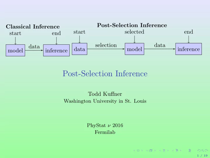
Classical Inference model start inference end data Post-Selection Inference data start model selected inference end selection data

Post-Selection Inference

Todd Kuffner

Washington University in St. Louis PhyStat ν 2016 Fermilab

1 / 19

Setting the mood

Cupua¸ cu and Octavia

2 / 19

Preliminary Comment: the p-value controversy (K-Walker 2016)

2015 Basic and Applied Social Psychology bans use of p-values (Trafimow & Marks, 2015) ‘fails to provide the probability of the null hypothesis, which is needed to provide a strong case for rejecting it’

3 / 19

Preliminary Comment: the p-value controversy (K-Walker 2016)

2015 Basic and Applied Social Psychology bans use of p-values (Trafimow & Marks, 2015) ‘fails to provide the probability of the null hypothesis, which is needed to provide a strong case for rejecting it’ 2015 International Society for Bayesian Analysis doesn’t gloat! (Bulletin, March 2015) ‘it was inspired by a nihilistic anti-statistical stance, backed by an apparent lack of understanding of the nature of statistical inference, rather than a call for saner and safer statistical practice’ (Christian P. Robert)

3 / 19

Preliminary Comment: the p-value controversy (K-Walker 2016)

2015 Basic and Applied Social Psychology bans use of p-values (Trafimow & Marks, 2015) ‘fails to provide the probability of the null hypothesis, which is needed to provide a strong case for rejecting it’ 2015 International Society for Bayesian Analysis doesn’t gloat! (Bulletin, March 2015) ‘it was inspired by a nihilistic anti-statistical stance, backed by an apparent lack of understanding of the nature of statistical inference, rather than a call for saner and safer statistical practice’ (Christian P. Robert) 2016 American Statistical Association (Wasserstein & Lazar, 2016) ‘Informally, a p-value is the probability under a specified statistical model that a statistical summary of the data . . . would be equal to or more extreme than its observed value.’

3 / 19

What is a p-value? The setting

Given X = {X1, . . . , Xn} (i.i.d.). Goal: test H S(X) =sufficient statistic; for simplicity assume dim(S(X)) = 1 ⇒ e.g. S(X) takes values in R Two decisions: R or RC ⇒ real line split into regions R and RC S(X) ∈ R

• r S(X) ∈ RC

Let α ∈ (0, 1), and define Rα ≡ R(α); for simplicity, assume Rα of form [cα, ∞) ⇒ test rejects H if S(X) ≥ cα

4 / 19

The Formal Definition of a p-value

p-value defined in setting where rejection regions are nested sets α < α′ ⇒ Rα ⊂ Rα′ Definition: The p-value, p ≡ ˆ α, is (Lehmann & Romano, 2005, §3.3) ˆ α ≡ ˆ αS(X) = inf

0<α<1{α : S(X) ∈ Rα}.

The p-value function, ˆ α = f(S(X)), for suitable map f : S(X) → ˆ α is a bijection from R to (0, 1) A p-value is not itself defined as a probability, but rather takes values on the same scale as something formally defined as a probability.

5 / 19

For the curious

Goal: show that the p-value, ˆ α = f(S(X)) for suitable choice of map f : S(X) → ˆ α, is a bijection from R to (0, 1). The actual form of ˆ α = f(S(X)) is specific to the model, hypothesis and test. Write S ≡ S(X) for simplicity. Step 1 First, we note that the function ˆ α is well-defined. That is, given two values S1, S2 such that S1 = S2, we have that ˆ αS1 = ˆ αS2. Step 2 Next, we require that ˆ α is injective (one-to-one). To show this, we need that if ˆ αS1 = ˆ αS2, then S1 = S2. Suppose that S1 = S2. If we can show that this implies ˆ αS1 = ˆ αS2, this will establish injectivity. Without loss of generality, suppose S2 < S1. Then there exists an α′ such that S1 ∈ Rα′ but S2 / ∈ Rα′. Therefore, if S2 < S1, it cannot be the case that ˆ αS1 = ˆ αS2. Step 3 Finally, we must have that ˆ α is surjective (onto). For surjectivity, we require that for every β ∈ (0, 1), there exists an ˜ S ∈ R such that ˆ α = inf

0<α<1{α : ˜

S ∈ Rα} = β, which is seen by choosing ˜ S = inf{S : S ∈ Rβ}.

6 / 19

Example

Suppose X = X1, . . . , Xn

i.i.d.

∼ N(θ, 1).

7 / 19

Example

Suppose X = X1, . . . , Xn

i.i.d.

∼ N(θ, 1). Wish to test H : θ = 0.

7 / 19

Example

Suppose X = X1, . . . , Xn

i.i.d.

∼ N(θ, 1). Wish to test H : θ = 0. Assume type I error probability α set in advance.

7 / 19

Example

Suppose X = X1, . . . , Xn

i.i.d.

∼ N(θ, 1). Wish to test H : θ = 0. Assume type I error probability α set in advance. S(X) = ¯ X = n−1 n

i=1 Xi

7 / 19

Example

Suppose X = X1, . . . , Xn

i.i.d.

∼ N(θ, 1). Wish to test H : θ = 0. Assume type I error probability α set in advance. S(X) = ¯ X = n−1 n

i=1 Xi

p-value assigns value in (0, 1) to each value in sample space of ¯ X

7 / 19

Example

Suppose X = X1, . . . , Xn

i.i.d.

∼ N(θ, 1). Wish to test H : θ = 0. Assume type I error probability α set in advance. S(X) = ¯ X = n−1 n

i=1 Xi

p-value assigns value in (0, 1) to each value in sample space of ¯ X p-value is merely transformation of ¯ X ⇒ p-value also sufficient for test

7 / 19

Example

Suppose X = X1, . . . , Xn

i.i.d.

∼ N(θ, 1). Wish to test H : θ = 0. Assume type I error probability α set in advance. S(X) = ¯ X = n−1 n

i=1 Xi

p-value assigns value in (0, 1) to each value in sample space of ¯ X p-value is merely transformation of ¯ X ⇒ p-value also sufficient for test Rejecting use of p-value conceptually equivalent to rejecting use of ¯ X

7 / 19

Source of the controversy: no decision rule

Three types of ‘testers’:

8 / 19

Source of the controversy: no decision rule

Three types of ‘testers’: Tester 1 sets α before seeing data; computes observed value of p based on sample, rejects H if p < α

8 / 19

Source of the controversy: no decision rule

Three types of ‘testers’: Tester 1 sets α before seeing data; computes observed value of p based on sample, rejects H if p < α Tester 2 first computes observed value of p, then claims his/her α would have been bigger had he/she actually chosen one beforehand

8 / 19

Source of the controversy: no decision rule

Three types of ‘testers’: Tester 1 sets α before seeing data; computes observed value of p based on sample, rejects H if p < α Tester 2 first computes observed value of p, then claims his/her α would have been bigger had he/she actually chosen one beforehand Tester 3 first computes observed value of p, believes it is small, and subsequently rejects H; he/she believes α is actually the

• bserved value of p, since following Tester 2’s approach, any

α > p will work; therefore, he/she argues: why not choose an α just above p and view that as the type I error probability?

8 / 19

Source of the controversy: no decision rule

Three types of ‘testers’: Tester 1 sets α before seeing data; computes observed value of p based on sample, rejects H if p < α Tester 2 first computes observed value of p, then claims his/her α would have been bigger had he/she actually chosen one beforehand Tester 3 first computes observed value of p, believes it is small, and subsequently rejects H; he/she believes α is actually the

• bserved value of p, since following Tester 2’s approach, any

α > p will work; therefore, he/she argues: why not choose an α just above p and view that as the type I error probability? For Testers 2 and 3, there is no decision rule; instead a heuristic: that small value of p is sufficient to reject the hypothesis.

8 / 19

The problem of post-selection inference

Classical inference assumes the model is chosen independently of the data.

9 / 19

The problem of post-selection inference

Classical inference assumes the model is chosen independently of the data. Using the data to select the model introduces additional uncertainty ⇒ invalidates classical inference

9 / 19

The problem of post-selection inference

Classical inference assumes the model is chosen independently of the data. Using the data to select the model introduces additional uncertainty ⇒ invalidates classical inference Do you believe me?

9 / 19

Example

• R. Lockhart, J. Taylor, Ryan Tibshirani, Rob Tibshirani (2014), ‘A

significance test for the lasso’, Annals of Statistics. Classical inference for linear regression: two fixed, nested models Model A variable indices M ⊂ {1, . . . , p} Model B variable indices M ∪ {j} Goal: test significance of jth predictor in Model B Compute drop in RSS from regression on M ∪ {j} and M Rj = (RSSM − RSSM∪{j})/σ2 versus χ2

1

• for σ2 known

10 / 19

Post-selection inference: first use selection procedure, then do inference want to do the same test as above for Models A and B which are not fixed, but rather outputs of selection procedure e.g. forward stepwise start with empty model M = ∅ enter predictors one at a time: choose predictor j giving largest drop in RSS FS chooses j at each step to to maximize Rj = (RSSM − RSSM∪{j})/σ2 each Rj ∼ χ2

1 (under null)

⇒ max possible Rj stochastically larger than χ2

1 under null

11 / 19

Illustration

Compare quantiles of R1 in forward stepwise regression, i.e. chi-square for first predictor to enter versus those of χ2

1 variable, when βk = 0 ∀k = 1, . . . , p.

n = 100, p = 10 (orthogonal); all true coefficients are zero; 1000 simulations of statistic R1, versus χ2

1 distribution; dotted line is 0.95 quantile of χ2 1

At 0.05 level, using χ2

1 quantile (3.84) has actual type I error probability of 0.39

12 / 19

Example: File Drawer Effect (Fithian, 2015)

Observe X1, . . . , Xn independently ∼N(µi, 1) Suppose you focus on ‘apparently’ large effects, |Xi| > 1: ˆ I = {i : |Yi| > 1} Goal: test H0,i : µi = 0 for each i ∈ ˆ I at level 0.05. Usual approach: reject H0,i when |Yi| > 1.96 Not Valid Due to Selection Why? Seems counterintuitive: probability of falsely rejecting a given H0,i is still α, since most of the time H0,i is not tested at all. Problem: for those hypotheses selected for testing, type I error rate is possibly much higher than α

13 / 19

Proof of concept

let n0 be # of true null effects assume n0 → ∞ as n → ∞ Long-run fraction of errors among the true nulls we test: # false rejections # true nulls selected =

1 n0

• i:H0,i true

1{i ∈ ˆ I, reject H0,i}

1 n0

• i:H0,i true

1{i ∈ ˆ I} → PH0,i(i ∈ ˆ I, reject H0,i) P(i ∈ ˆ I) = PH0,i(reject H0,i | i ∈ ˆ I) For nominal test, this is Φ(−1.96)/Φ(−1) ≈ 0.16

14 / 19

Why should particle physicists care?

We hate false discovery as much as you do. control of FDR, FCR, FWER are key desiderata in PSI applications are endless: need to formalize the informal ‘data snooping’ (adaptive selection) process to properly account for uncertainty Possible problems? select minimum signal threshold, then do inference for selected signals selection of ‘events’ data transformations based on data snooping

15 / 19

Broad Classification of PSI

• 1. data splitting (Cox, Wasserman) and data carving (Fithian)

idea: the source of the problem is using the same data for selection and inference; solution: use some data for selection, the rest for inference

• 2. high-dimensional inference (the Swiss, signal processing, machine

learning, econometrics): idea: ignore selection, view as single procedure followed by interval correction; not really PSI?

• 3. simultaneous inference (Benjamini, Yekutieli, Heller, Wharton)

idea: control FDR for all models ever under consideration by selection procedure; solution: fix the confidence intervals

• 4. selective inference (Benjamini, Yekutieli, Stanford)

idea: inference for selected hypotheses

16 / 19

Point of Contention

Suppose we have Full model: Yi =

p

• k=1

βikxik + εi Apply selection procedure, result is Selected/sub- model: Yi =

• k∈ ˆ

M

βikxik + γi with ˆ M ⊆ {1, . . . , p}. Parameter spaces are not the same; should we do inference about full model parameters or submodel parameters?

17 / 19

More on Selective Inference

The selection of a model is a random event. helpful toy example: the set of selected variables in regression is a random set; hypotheses are only tested for selected variables, thus the hypotheses are random to condition on selection event, need to characterize this event in a manner suitable to uncertainty quantification e.g. Lasso and forward stepwise partition Rn into convex polyhedra: if y ∈ ConvPolym, then model m is selected

18 / 19

Are Bayesians immune?

Dawid (1994): selection should have no effect Since Bayesian posterior distributions are already fully conditioned

• n the data, the posterior distribution of any quantity is the same,

whether it was chosen in advance or selected in the light of the data. Yekutieli (2012, ‘Adjusted Bayesian inference for selected parameters,’ JRSSB): Actually, selection can affect Bayesian inference

Bayesian inference for parameters selected after viewing the data is a ‘truncated’ data problem.

19 / 19