Image Domain Gridding Sebastiaan van der Tol, Bram Veenboer - PowerPoint PPT Presentation

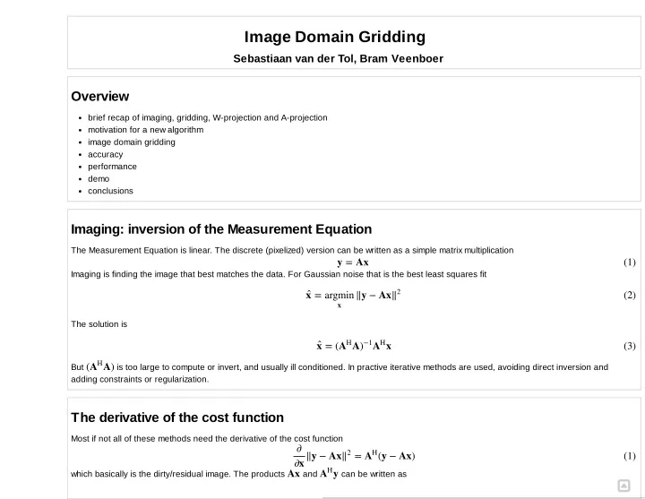
Image Domain Gridding Sebastiaan van der Tol, Bram Veenboer Overview brief recap of imaging, gridding, W­projection and A­projection motivation for a new algorithm image domain gridding accuracy performance demo conclusions Imaging: inversion of the Measurement Equation The Measurement Equation is linear. The discrete (pixelized) version can be written as a simple matrix multiplication y = Ax (1) Imaging is finding the image that best matches the data. For Gaussian noise that is the best least squares fit ‖ 2 x ̂ = argmin ‖ y − Ax (2) x The solution is A H ) − 1 A H x ̂ = ( A x (3) But is too large to compute or invert, and usually ill conditioned. In practive iterative methods are used, avoiding direct inversion and A H ( A ) adding constraints or regularization. The derivative of the cost function Most if not all of these methods need the derivative of the cost function ∂ ‖ 2 A H ‖ y − Ax = ( y − Ax ) (1) ∂ x which basically is the dirty/residual image. The products and can be written as A H Ax y  N N

N N e − 2 π j( u pqk l i + v pqk m j w pqk n ij J pijk B ij J H + ) V pqk = (2) qijk ∑ ∑ i =1 j =1 . e 2 π j( u pqk l i + v pqk m j w pqk n ij J H + ) I ij = pijk V pq J qijk (3) ∑ k =1 ∑ p =1 ∑ q =1 Gridding, Degridding, W projection and A Projection Computing visibilities and pixels this way is expensive because each pixel is the sum of all visibilities and each predicted visibility is the sum of all (non­zero) pixels of the model image. The solution is of course well known. These equation resemble the Discrete Fourier Transform, which can be computed very efficiently. For this to work the measured visibility need to be on a regular grid, which they aren't. The trick is to resample the data from or to a regular grid using convolutional resampling. The convolution kernel is an anti­aliasing filter, but it can also include other effects, like the W term and the beam/ A term Motivation for a new algorithm: AWImager + ionosphere The convolution kernel is computed on an oversampled grid. The taper, w­term and a­term are computed in the image domain and then zero padded by the required oversampling factor, and then Fourier transformed. When the a­term is varying over very short times scales, which is the case when ionospheric effects are included, the computation of the convolution kernels becomes much more expensive then the subsequent gridding operation itself. Image Domain Gridding Idea: why not pull the gridding operation to the image domain, instead of bringing the convolution kernel to the uv domain? But wait: we moved the operations from the image domain to the uv domain because it is more efficient. If we move the operation back to the image domain again, aren't we then back to the DFT. Well, almost, but not quite. The difference is that we operare on far fewer pixels, because we select only a small region in the uvdomain. UV tracks

Partitioning the visibilities

UV Subgrid encompassing all affected pixels

Equation for the subgrid Selecting a subgrid shifts origin of Fourier transform to center of subgrid. N N

N N e − 2 π j(( u pqk u 0 l i − ) +( v pqk − v 0 m j w pqk n ij J pijk B ij J H ) + ) V pqk = ∑ qijk W ij (7) ∑ i =1 j =1 e 2 π j(( u pqk u 0 l i − ) +( v pqk − v 0 m j w pqk n ij J H ) + ) I ij = ∑ pijk V pq J qijk W ij (8) k =1 Gridding flow diagram Degridding flow diagram

Effective operation in the uv domain

Effective operation in the image domain ⃛ ˜ ̂ = [ ( , ) ( , )]( , )

I ⃛ ˜ y ̂ =  [ ( l , m ) W ( l , m )]( u , v ) where is the infinitely repeated model image I ⃛ ( l , m ) and is the sinc interpolated window. ˜ W ( l , m ) Error compared to classical gridding with PSWF W PSWF N=8 N=16 N=24 N=32 N=48 N=64 3.0 3.33e­02 4.63e­02 2.87e­02 2.25e­02 1.92e­02 1.54e­02 1.32e­02 5.0 1.68e­03 4.60e­03 2.59e­03 1.94e­03 1.60e­03 1.25e­03 1.06e­03 7.0 7.96e­05 2.99e­04 1.67e­04 1.25e­04 1.03e­04 7.89e­05 6.62e­05 9.0 3.68e­06 9.08e­06 6.96e­06 5.78e­06 4.45e­06 3.71e­06 11.0 1.68e­07 4.82e­07 3.55e­07 2.98e­07 2.33e­07 1.95e­07 13.0 7.58e­09 2.70e­08 1.79e­08 1.47e­08 1.16e­08 9.83e­09 15.0 3.40e­10 1.45e­09 9.15e­10 7.25e­10 5.61e­10 4.78e­10 Error as function position in subgrid Error as function of position in image

Error as function of position in image Subgrid pixel budget Tapering window 7 W term 8 A term 8 UV coverage 9

Computational Properties very regular structure with lots of paralellism fewer access to memory, because there is no lookup in a sampled convolution function But touches many more pixels per visibility, typically 32x32 vs 7x7 classical gridding and needs to evaluate a sincos per pixel Well suited for a GPU with sincos hardware instruction Implementation Bram Veenboer Ph.D. Researcher ASTRON (Netherlands Institute for Radio Astronomy) DOME Project (ASTRON + IBM) High Performance Computing Implementations for different platforms: CPU, Xeon Phi, CUDA, OpenCL It provides a python interface and a c++ interface git clone git@gitlab.com:astron­idg/code.git (not for commercial use, patent pending) CPU Demo in laptop

In [6]: ! NR_TIME=256 cpu ­ optimized.x >>> Configuration ­­­­­­­­­­­ PARAMETERS: Number of stations == 44 Number of baselines == 946 Number of channels == 8 Number of time == 256 Number of timeslots == 16 Imagesize == 0.1 Grid size == 1024 Subgrid size == 32 Job size == 256 Job size (gridding) == 256 Job size (degridding) == 256 Job size (gridder) == 256 Job size (adder) == 256 Job size (splitter) == 256 Job size (degridder) == 256 ­­­­­­­­­­­ CPU Demo on compute node 2x Xeon E5­2660v3, 20 cores, 40 threads

In [7]: ! ssh node505 SUBGRIDSIZE=32 NR_TIMESLOTS=32 . / cpu ­ demo.sh cpu­demo >>> Configuration ­­­­­­­­­­­ PARAMETERS: Number of stations == 44 Number of baselines == 946 Number of channels == 8 Number of time == 4096 Number of timeslots == 32 Imagesize == 0.1 Grid size == 4096 Subgrid size == 32 Job size == 256 Job size (gridding) == 256 Job size (degridding) == 256 Job size (gridder) == 256 Job size (adder) == 256 Job size (splitter) == 256 Job size (degridder) == 256 ­­­­­­­­­­­ GPU demo on laptop

In [8]: ! cuda ­ generic.x >>> Configuration ­­­­­­­­­­­ PARAMETERS: Number of stations == 44 Number of baselines == 946 Number of channels == 8 Number of time == 4096 Number of timeslots == 16 Imagesize == 0.1 Grid size == 1024 Subgrid size == 32 Job size == 256 Job size (gridding) == 256 Job size (degridding) == 256 Job size (gridder) == 256 Job size (adder) == 256 Job size (splitter) == 256 Job size (degridder) == 256 ­­­­­­­­­­­ GPU demo on a compute node

In [14]: ! ssh node505 SUBGRIDSIZE=32 NR_TIME=32000 . / gpu ­ demo.sh gpu­demo >>> Configuration ­­­­­­­­­­­ PARAMETERS: Number of stations == 44 Number of baselines == 946 Number of channels == 8 Number of time == 32000 Number of timeslots == 16 Imagesize == 0.1 Grid size == 4096 Subgrid size == 32 Job size == 256 Job size (gridding) == 256 Job size (degridding) == 256 Job size (gridder) == 256 Job size (adder) == 256 Job size (splitter) == 256 Job size (degridder) == 256 ­­­­­­­­­­­ Demo python interface

In [2]: % matplotlib inline from common import * main(idg.CUDA.Generic) nr_stations = 12 nr_baselines = 66 nr_channels = 8 nr_timesteps = 4096 nr_timeslots = 8 nr_polarizations = 4 subgrid_size = 32 grid_size = 1024 image_size = 0.0599999986589 kernel_size = 17 job size (gridding) = 256 job size (degridding) = 256