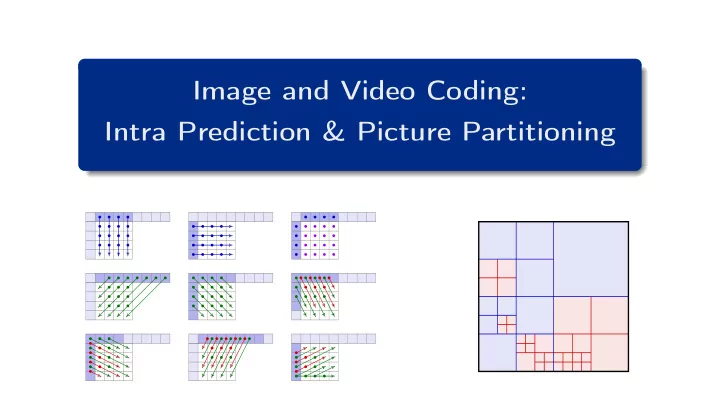
Image and Video Coding: Intra Prediction & Picture Partitioning - - PowerPoint PPT Presentation

Image and Video Coding: Intra Prediction & Picture Partitioning

Intra-Picture Prediction

Transform Coding with Intra-Picture Prediction

sample array

2d block transform quantization entropy coding bitstream

• riginal

8×8 block bits

Transform Coding of Sample Blocks Decorrelating transform: Utilization of statistical dependencies (correlations) inside blocks There are also statistical dependencies between transform blocks Exploitation of these inter-block dependencies can increase coding efficiency

• riginal picture

(256×256) averages of 16×16 blocks (DC coefficients) example: DC coefficients

Heiko Schwarz (Freie Universität Berlin) — Image and Video Coding: Intra Prediction & Picture Partitioning 2 / 35

Intra-Picture Prediction / Prediction of Transform Coefficients

Prediction of DC Coefficient (JPEG, MPEG-2 Video)

Prediction of DC Quantization Index DC (direct current) represents scaled average of block samples (often similar to DC of neighboring blocks) Prediction using DC quantization index of block to the left Prediction difference DIFF = DCk − DCk−1 is entropy coded Improves coding efficiency

block k − 1 block k DCk−1 DCk DIFF = DCk − DCk−1

quantization: ∆ = 8

P( DC − N 2B−1/∆)

σ = 37.0 H = 6.01

P( DIFF )

σ = 5.29 H = 3.10

Heiko Schwarz (Freie Universität Berlin) — Image and Video Coding: Intra Prediction & Picture Partitioning 3 / 35

Intra-Picture Prediction / Prediction of Transform Coefficients

Example: Coding Efficiency Impact of DC Prediction (8×8 Blocks)

26 28 30 32 34 36 38 40 42 44 46 0.5 1 1.5 2 2.5 3 3.5 4

17 % 29 %

Luma PSNR [dB] bits per luma sample Berlin (1200 x 900) without prediction with DC prediction

Heiko Schwarz (Freie Universität Berlin) — Image and Video Coding: Intra Prediction & Picture Partitioning 4 / 35

Intra-Picture Prediction / Prediction of Transform Coefficients

Additional Dependencies between Transform Coefficients

T T Mainly Horizontal Structures

Signal energy is concentrate in first column of transform coefficients Horizontal neighboring blocks have similar first column of transform coefficients

Mainly Vertical Structures

Signal energy is concentrate in first row of transform coefficients Vertical neighboring blocks have similar first row of transform coefficients

T T

Heiko Schwarz (Freie Universität Berlin) — Image and Video Coding: Intra Prediction & Picture Partitioning 5 / 35

Intra-Picture Prediction / Prediction of Transform Coefficients

Advanced Intra Prediction in Transform Domain (H.263, MPEG-4 Visual)

Prediction of transform coefficients t using reconstructed transform coefficients t′ Quantization of prediction error ∆t = t − ˆ t

ˆ t0,0 = a′

0,0 + b′ 0,0

2

a b

∀y : ˆ t0,y = a′

0,y

∀x : ˆ tx,0 = b′

x,0

Three Intra Coding Modes

1 DC mode:

Prediction of DC coefficient and zig-zag scan

2 Horizontal mode:

Prediction of first column (from left block) and alternate-vertical scan

3 Vertical mode:

Prediction of first row (from above block) and alternate-horizontal scan

Heiko Schwarz (Freie Universität Berlin) — Image and Video Coding: Intra Prediction & Picture Partitioning 6 / 35

Intra-Picture Prediction / Prediction of Transform Coefficients

How to Select Suitable Coding Mode?

Intra Mode Selection Syntax supports multiple intra prediction modes (mode is transmitted) Encoder has to select one of the supported modes Goal: Maximize coding efficiency Lagrangian Mode Decision

1 Transform original block of samples 2 Evaluate all supported coding modes (DC, horizontal, vertical)

Perform prediction, quantization, and reconstruction of transform coefficient Calculate SSD distortion D =

k (t′ k − tk)2

Determine number of bits R for transmitting mode and block of quantization indexes

3 Select intra mode m that minimizes Lagrangian cost function

Jm = Dm + λ · Rm

Heiko Schwarz (Freie Universität Berlin) — Image and Video Coding: Intra Prediction & Picture Partitioning 7 / 35

Intra-Picture Prediction / Spatial Intra Prediction

Intra Prediction: Transform Domain or Spatial Domain ?

vertical prediction in transform domain ˆ t[x, 0] = t′

above[x, 0]

equivalent prediction in spatial domain ˆ s[x, y] = 1 N

N

• k=1

s′[x, −k] simplified and improved vertical prediction in spatial domain ˆ s[x, y] = s′[x, −1]

Intra Prediction in Transform Domain Disadvantage: Only possible if neighboring block is intra-coded (problem in video pictures) Intra Prediction in Spatial Domain Similar complexity than similar prediction in transform domain Usage of directly adjacent samples improves coding efficiency Main Advantages: Can also be applied if neighboring blocks are coded in an inter mode Straightforward extension to multiple prediction directions

Heiko Schwarz (Freie Universität Berlin) — Image and Video Coding: Intra Prediction & Picture Partitioning 8 / 35

Intra-Picture Prediction / Spatial Intra Prediction

Spatial Intra Prediction in H.264 | MPEG-4 AVC (for 4×4 Blocks)

vertical prediction −90◦ horizontal prediction 0◦ =

• 8
• DC prediction

average diagonal down-left prediction −135◦ diagonal down-right prediction −45◦ vertical-right prediction −63.4◦ horizontal-down prediction −27.6◦ vertical-left prediction −117.6◦ horizontal-up prediction 27.6◦ a = a a b c =

• a + 2b + c + 2
• ≫ 2

a b =

• a + 3b + 2
• ≫ 2

a b =

• a + b + 1
• ≫ 1

similar 9 modes for 8×8 blocks (with additional border smoothing); 4 modes for 16×16 blocks (DC, hor., ver., plane)

Heiko Schwarz (Freie Universität Berlin) — Image and Video Coding: Intra Prediction & Picture Partitioning 9 / 35

Intra-Picture Prediction / Spatial Intra Prediction

Spatial Intra Prediction in H.265 | MPEG-H HEVC

Intra Prediction in H.265 | MPEG-H HEVC Unique intra prediction for all block sizes (4×4 to 32×32) 35 spatial intra prediction modes 33 directional prediction modes (slopes of k/32) DC prediction mode (similar to H.264 | AVC) Planar prediction mode (smooth prediction signal)

DC prediction mode:

=

• 1

2N

• N +
• 45◦

−135◦

32

• 32
• 32

32 Heiko Schwarz (Freie Universität Berlin) — Image and Video Coding: Intra Prediction & Picture Partitioning 10 / 35

Intra-Picture Prediction / Spatial Intra Prediction

Angular Intra Prediction in H.265 | MPEG-H HEVC

example: mode 21

linear interpolation between neighboring border samples

Mainly vertical modes (modes 18 – 34)

1 Fill not existing border samples

Replace with closest existing border sample

2 Filtering of border samples

Typically: Use (1,2,1) filter (as in H.264) No filtering for close to vertical modes

3 Create virtual top border

Copy from left border in prediction direction

4 Predict samples from virtual top border

Predict from virtual top border in prediction direction (using linear interpolation)

Mainly horizontal modes (modes 2 – 17) Same signal processing (for transposed data)

No filtering for close to horizontal modes Use virtual left border

Heiko Schwarz (Freie Universität Berlin) — Image and Video Coding: Intra Prediction & Picture Partitioning 11 / 35

Intra-Picture Prediction / Spatial Intra Prediction

Planar Prediction Mode in H.265 | MPEG-H HEVC

Basic Idea Not all blocks fit an directional model DC mode: Coarse approximation (order 0) Planar mode: Smooth approximation

Bilinear interpolation of sample values Linear interpolated right-bottom border ˆ sx,y = bilinear

• L′

y, T ′ x, R∗ y , B∗ x

• R∗

y = linear

• T ′

N−1, C ∗

B∗

y = linear

• L′

N−1, C ∗

C ∗ = 1 2

• T ′

N−1 + L′ N−1

• Planar Mode in HEVC

Simplified design without border interpolation

ˆ h[x, y] = (N−1−x) · s′[−1, y] + (1+x) · s′[N−1, −1] ˆ v[x, y] = (N−1−y) · s′[x, −1] + (1+y) · s′[−1, N−1] ˆ s[x, y] = 1 2N

• ˆ

h[x, y] + ˆ v[x, y]

• copy

copy

Heiko Schwarz (Freie Universität Berlin) — Image and Video Coding: Intra Prediction & Picture Partitioning 12 / 35

Intra-Picture Prediction / Spatial Intra Prediction

Illustration of Intra Prediction Modes in H.265 | MPEG-H HEVC

?

35 intra prediction modes: 0: planar mode 1: DC mode 2: angular mode (+45◦) · · · 10: angular mode (0◦): horizontal · · · 18: angular mode (−45◦) · · · 26: angular mode (−90◦): vertical · · · 34: angular mode (−135◦)

2 10

. . .

18

. . .

26

· · ·

34

· · ·

Heiko Schwarz (Freie Universität Berlin) — Image and Video Coding: Intra Prediction & Picture Partitioning 13 / 35

Intra-Picture Prediction / Modern Intra-Picture Coding

Selection of Spatial Intra Prediction Mode for a Given Block

Lagrangian Mode Decision For all possible intra prediction modes p :

1 Generate block prediction signal ˆ

sp[x, y] using mode p

2 Transform encoding and decoding of prediction residual up[x, y] = s[x, y] − ˆ

sp[x, y]

includes transform, quantization, dequantization, and inverse transform 3 Reconstruct block s′

p[x, y] = ˆ

sp[x, y] + u′

p[x, y]

4 Calculate SSD distortion D(p) =

x,y( s[x, y] − s′ p[x, y] )2

5 Determine number of bits R(p) for entropy coding of mode p and quantization indexes qp[x, y]

Select intra prediction mode that minimizes Lagrangian cost J(p) = D(p) + λ · R(p) Fast Mode Decision Strategies (typical approach)

1 Select candidate set (e.g., 5 modes) based on simple measure (such as prediction error) 2 Select final mode out of candidate set using Lagrangian mode decision

Heiko Schwarz (Freie Universität Berlin) — Image and Video Coding: Intra Prediction & Picture Partitioning 14 / 35

Intra-Picture Prediction / Modern Intra-Picture Coding

Modern Image Coding: Encoder Structure

partitioned into blocks

• 2d block

transform scalar quantization entropy coding “inverse” quantization inverse transform intra-picture prediction predictor selection

sn[x, y] un[x, y] tn[x, y] qn[x, y]

bitstream

t′

n[x, y]

u′

n[x, y]

s′

n[x, y]

s′

pic[x, y]

− ˆ sn[x, y] moden sn[x, y] s′

pic[x, y]

moden

Heiko Schwarz (Freie Universität Berlin) — Image and Video Coding: Intra Prediction & Picture Partitioning 15 / 35

Intra-Picture Prediction / Modern Intra-Picture Coding

Modern Image Coding: Decoder Structure

entropy decoding “inverse” quantization inverse transform intra-picture prediction

qn[x, y]

bitstream

t′

n[x, y]

u′

n[x, y]

s′

n[x, y]

s′

pic[x, y]

ˆ sn[x, y]

• utput

moden

Heiko Schwarz (Freie Universität Berlin) — Image and Video Coding: Intra Prediction & Picture Partitioning 16 / 35

Intra-Picture Prediction / Modern Intra-Picture Coding

Coding Efficiency Impact of Spatial Intra Prediction

10 20 30 40 50 30 32 34 36 38 40 DC, horizontal, vertical (avg. 11%) 9 prediction modes (avg. 14%) all 35 prediction modes (avg. 25%) bit-rate saving vs DC pred. [%] PSNR (Y) [dB] Cactus (1920×1080, 50 Hz), 8×8 blocks 10 20 30 40 50 34 36 38 40 42 44 DC, horizontal, vertical (avg. 9%) 9 prediction modes (avg. 14%) all 35 prediction modes (avg. 25%) bit-rate saving vs DC pred. [%] PSNR (Y) [dB] Kimono (1920×1080, 24 Hz), 8×8 blocks

Experimental Investigation with H.265 | MPEG-H HEVC Restricted to 8×8 blocks (effect of block size is discussed later) Compare multiple intra prediction mode to DC prediction only Coding efficiency increases with number of supported intra prediction modes

Heiko Schwarz (Freie Universität Berlin) — Image and Video Coding: Intra Prediction & Picture Partitioning 17 / 35

Intra-Picture Prediction / Intra Prediction Improvements in VVC

Spatial Intra Prediction in H.266 | VVC

Spatial Intra Prediction in H.266 | VVC 67 spatial intra prediction modes DC mode and planar mode (as in HEVC) 65 directional prediction modes (HEVC has 33) Wide angle prediction directions (no non-square blocks) Only 65 (out of 93) directions available per block shape

conventional directions (45◦ to −135◦) wide angle directions (for 3:1 blocks)

32

• 32
• 32

32 Heiko Schwarz (Freie Universität Berlin) — Image and Video Coding: Intra Prediction & Picture Partitioning 18 / 35

Intra-Picture Prediction / Intra Prediction Improvements in VVC

H.266 | VVC: Modifications of Conventional Intra Prediction

Position Dependent Prediction Sample Filtering Prediction refinement for selected modes Linear combination of unfiltered border samples and conventional prediction signals ˆ sx,y = wx ·Ly + wy ·Tx + (1−wx −wy)·ˆ s∗

x,y

wx wy

planar DC

wy wx = 0 wx wy = 0

Multi Reference Line Intra Prediction Directly neighboring samples are not always the best choice for intra prediction Block-adaptive selection of border samples used

directly neighboring border samples border samples in a distance of 1 border samples in a distance of 3

idx = 0 1 2

Heiko Schwarz (Freie Universität Berlin) — Image and Video Coding: Intra Prediction & Picture Partitioning 19 / 35

Intra-Picture Prediction / Intra Prediction Improvements in VVC

Additional Modes in H.266 | VVC: Matrix-based Intra Prediction

?

r p = Ak ·r + bk

mode k

New Matrix-based Intra Prediction Modes (luma only) Original Idea: Learned intra prediction modes (using neural network) Simplified version in VVC

1 Downsampling of border samples yielding reference samples r 2 Matrix-vector multiplication yielding sparse prediction samples p 3 Generation of final prediction signal using linear interpolation

Three sets of up to 16 additional intra prediction modes k (matrices Ak and vectors bk)

Heiko Schwarz (Freie Universität Berlin) — Image and Video Coding: Intra Prediction & Picture Partitioning 20 / 35

Intra-Picture Prediction / Intra Prediction Improvements in VVC

Intra Prediction of Chroma Components in H.266 | VVC

Intra Prediction of Chroma Samples Same spatial prediction modes as for luma Only 5 possible modes per block (same for both components)

mode of co-located luma block, horizontal, vertical, planar, DC

Cross-Component Linear Model Prediction (CCLM) Downsampling of reconstructed luma signal s′

L[x, y] → s∗ L[x, y]

Chroma samples are predicted using downsampled luma signal ˆ sC[x, y] = α · s∗

L[x, y] + β

Parameters α and β are determined by regression using reconstructed chroma border b′

C and luma border b∗ L

mode 0: top and left border mode 1:

• nly left border

mode 2:

• nly top border

s′

L[x, y]

b′

L

downsampling

s∗

L[x, y]

b∗

L

ˆ sC[x, y] b′

C

Heiko Schwarz (Freie Universität Berlin) — Image and Video Coding: Intra Prediction & Picture Partitioning 21 / 35

Picture Partitioning

Impact of Block Size on Coding Efficiency

4×4 blocks: 27.7 dB @ 0.3 bpp 16×16 blocks: 30.1 dB @ 0.3 bpp 64×64 blocks: 29.6 dB @ 0.3 bpp

Transform Coding: Coding efficiency increases with block size (for “stationary” blocks) Instationarities cause decrease of coding efficiency Intra Prediction: More effective for smaller blocks (correlation decreases with distance) Side information rate (prediction modes) is larger for smaller blocks Block size should be locally adapted (based on image properties)

Heiko Schwarz (Freie Universität Berlin) — Image and Video Coding: Intra Prediction & Picture Partitioning 22 / 35

Picture Partitioning / Variable Block Sizes

Block Sizes in Video Coding Standards up to H.264 | AVC

H.262 | MPEG-2 Video, H.263, MPEG-4 Visual Fixed block sizes for prediction and transform coding 16×16 macroblocks (for signaling intra prediction mode) and 8×8 transform blocks H.264 | MPEG-4 AVC (High profile) 16×16 macroblocks with 3 intra coding modes: Intra4x4, Intra8x8, Intra16x16 Block sizes for prediction and transform coding: 4×4, 8×8, 16×16 Intra prediction mode selected on basis of transform blocks

Intra4x4 Intra8x8 Intra16x16

Heiko Schwarz (Freie Universität Berlin) — Image and Video Coding: Intra Prediction & Picture Partitioning 23 / 35

Picture Partitioning / Variable Block Sizes

Picture Partitioning in H.265 | MPEG-H HEVC

Initial Partitioning of Pictures Partitioning into fixed-size blocks: Coding Tree Units (CTUs) CTU: 16×16, 32×32, or 64×64 luma samples Size of CTUs chosen by encoder (typically: 64×64) CTU includes co-located sample arrays of all color components Coding order of CTUs: Raster scan (line per line) Adaptive Refinement of Partitioning Quad-tree partitioning into Coding Units (CUs) CU includes co-located sample arrays of all color components Minimum CU size: Selected by encoder (≥ 8×8) Coding mode (intra or inter) is chosen for each CU Coding order of CUs: Z-scan

Heiko Schwarz (Freie Universität Berlin) — Image and Video Coding: Intra Prediction & Picture Partitioning 24 / 35

Picture Partitioning / Variable Block Sizes

Example: Picture Partitioning into Coding Units

Picture of test sequence “Traffic” (2560×1600 luma samples)

Heiko Schwarz (Freie Universität Berlin) — Image and Video Coding: Intra Prediction & Picture Partitioning 25 / 35

Picture Partitioning / Variable Block Sizes

Transform Coding and Intra Prediction in H.265 | MPEG-H HEVC

Transform Coding: Sub-Partitioning of CUs Quad-tree partitioning into Transform Units (TUs) Supported sizes: 32×32, 16×16, 8×8, and 4×4 TU: Co-located transform blocks for all color components

Minimum supported transform size: 4×4 samples Not all 4×4 TUs may include chroma blocks (for 4:2:2, 4:2:0)

Coding order of TUs: Z-scan Intra Prediction and Prediction Mode Coding Luma: One luma mode per CU Four modes per CU (only for minimum CU size) Chroma: One chroma mode per CU (for both components) Actual prediction is performed on transform blocks (improves prediction accuracy) m0

m0 m1 m2 m3

Heiko Schwarz (Freie Universität Berlin) — Image and Video Coding: Intra Prediction & Picture Partitioning 26 / 35

Picture Partitioning / Variable Block Sizes

Quadtree Partitioning: Coding Partitioning Data and Encoder Decision

CTU

1 1 1 1 1 1 1 1 1 1 1 1

Coding of Partitioning Data

CU Partitioning: Quadtree starting at CTU level cu_split_flag for each node TU Partitioning: Quadtree starting at CU level tu_split_flag for each node

Encoder Decision

Lagrangian mode decision (depth first order) Each node: Compare Lagrangian costs Jnosplit for non-split block Jsplit = Jsubblock for quad-tree split Potential subblocks and causal neighborhood are decided first

Heiko Schwarz (Freie Universität Berlin) — Image and Video Coding: Intra Prediction & Picture Partitioning 27 / 35

Picture Partitioning / Coding Efficiency Comparison

Coding Efficiency: Block Sizes for DC Prediction Only

30 32 34 36 38 40 20 40 60 80 100 4×4 blocks 8×8 blocks 16×16 blocks 32×32 blocks all block sizes PSNR (Y) [dB] bit rate [Mbit/s] Cactus (1920×1080, 50 Hz), DC prediction 34 36 38 40 42 44 10 20 30 40 50 4×4 blocks 8×8 blocks 16×16 blocks 32×32 blocks all block sizes PSNR (Y) [dB] bit rate [Mbit/s] Kimono (1920×1080, 24 Hz), DC prediction

H.265 | MPEG-H HEVC: Only DC Prediction Reduce impact of intra prediction: All blocks use DC prediction Fixed block sizes: Coding efficiency increases with block size Variable block sizes provide coding efficiency improvements

Heiko Schwarz (Freie Universität Berlin) — Image and Video Coding: Intra Prediction & Picture Partitioning 28 / 35

Picture Partitioning / Coding Efficiency Comparison

Coding Efficiency: Block Sizes for Multiple Intra Prediction Modes

30 32 34 36 38 40 20 40 60 80 100 4×4 blocks 8×8 blocks 16×16 blocks 32×32 blocks all block sizes PSNR (Y) [dB] bit rate [Mbit/s] Cactus (1920×1080, 50 Hz), all pred. modes 34 36 38 40 42 44 10 20 30 40 50 4×4 blocks 8×8 blocks 16×16 blocks 32×32 blocks all block sizes PSNR (Y) [dB] bit rate [Mbit/s] Kimono (1920×1080, 24 Hz), all pred. modes

H.265 | MPEG-H HEVC: All 35 Intra Prediction Modes Enabled Prediction increases effectiveness of smaller block sizes Fixed block sizes: Medium block sizes provide best coding efficiency Variable block sizes provide coding efficiency improvements

Heiko Schwarz (Freie Universität Berlin) — Image and Video Coding: Intra Prediction & Picture Partitioning 29 / 35

Picture Partitioning / Coding Efficiency Comparison

Coding Efficiency: Variable Block Sizes for Intra-Picture Coding

10 20 30 40 50 30 32 34 36 38 40 4×4 and 8×8 blocks: 11% 4×4, 8×8, and 16×16 blocks: 15% all block sizes (4×4 to 32×32): 18% bit-rate saving vs 8×8 blocks [%] PSNR (Y) [dB] Cactus (1920×1080, 50 Hz), all pred. modes 10 20 30 40 50 34 36 38 40 42 44 4×4 and 8×8 blocks: 9% 4×4, 8×8, and 16×16 blocks: 18% all block sizes (4×4 to 32×32): 23% bit-rate saving vs 8×8 blocks [%] PSNR (Y) [dB] Kimono (1920×1080, 24 Hz), all pred. modes

Experimental Investigation with H.265 | MPEG-H HEVC All 35 intra prediction mode are enabled Start with 8×8 blocks and successively enable additional block sizes Additional block sizes provide coding efficiency improvements

Heiko Schwarz (Freie Universität Berlin) — Image and Video Coding: Intra Prediction & Picture Partitioning 30 / 35

Picture Partitioning / Partitioning Improvements in VVC

Picture Partitioning in H.266 | VVC

Initial Partitioning of Pictures Partitioning into fixed-size Coding Tree Units (CTUs) CTU: 32×32, 64×64, or 128×128 luma samples CTU includes co-located sample arrays of all color components Coding order of CTUs: Raster scan (line per line) Adaptive Refinement of Partitioning Multi-Type Tree partitioning into Coding Units (CUs)

quad split (as in HEVC) binary split (horizontal or vertical) ternary split (horizontal or vertical)

Minimum CU width and height: 4 luma samples No additional partitioning tree for transform blocks

Heiko Schwarz (Freie Universität Berlin) — Image and Video Coding: Intra Prediction & Picture Partitioning 31 / 35

Picture Partitioning / Partitioning Improvements in VVC

Multi-Type Tree Partitioning in H.266 |VVC

split codeword no Q 1 1 Bh 1 0 0 1 Bv 1 0 1 1 Th 1 0 0 0 Tc 1 0 1 0

Multi-Type Tree Partitioning in VVC

CU can be sub-partitioned using one of 6 modes (no split, quad split, 2 binary splits, 2 ternary splits) Indicated by codeword for each node High-level parameters and several restrictions:

Binary/ternary split cannot be followed by quad split Width and height of blocks must be a multiple of 4 Avoidance of redundant split sequences

1 4 1 2 1 4

Th

1/4 1/2 1/4

Tv

1/2 1/2

Bh

1/2 1/2

Bv no

1/2 1/2

Q CTU

Q Bh Tv Q Bv Bv Tv Th Bh Q Th Bh no no no no no no no no no no no no no no no no no no no no no no no

Heiko Schwarz (Freie Universität Berlin) — Image and Video Coding: Intra Prediction & Picture Partitioning 32 / 35

Picture Partitioning / Partitioning Improvements in VVC

Intra-Picture Coding in H.266 | VVC

General Intra-Picture Coding Select one luma prediction mode per CU Select one chroma prediction mode per chroma CU (allows separate partitioning for chroma) Apply intra prediction and transform coding on CU basis Intra Sub-Partitioning Mode (luma only) Allows horizontal or vertical sub-partitioning of CU for intra prediction and transform coding Same intra prediction mode for all sub-partitions Advantage: Reduces distance to border samples used for prediction

4×8 or 8×4

hor ver

not 4×4, 4×8, or 8×4

hor ver

Heiko Schwarz (Freie Universität Berlin) — Image and Video Coding: Intra Prediction & Picture Partitioning 33 / 35

Coding Efficiency Comparison

Advanced Intra Coding: Impact on Coding Efficiency

30 31 32 33 34 35 36 37 38 39 40 41 42 0.5 1 1.5 2 Luma PSNR [dB] bits per luma sample Berlin (1200 x 900) JPEG (no RDOQ) H.264 | AVC H.265 | HEVC H.266 | VVC

additional VVC tools

multiple transforms non-separable transform dependent quantization

Heiko Schwarz (Freie Universität Berlin) — Image and Video Coding: Intra Prediction & Picture Partitioning 34 / 35

Summary

Summary of Lecture

Transform Coding of Sample Blocks Utilization only dependencies (correlations) inside blocks Intra-Picture Prediction Utilize dependencies between transform blocks Two methods: Prediction in transform domain or spatial domain Spatial prediction: Straightforward realization of multiple prediction modes Coding efficiency typically increases with number of supported intra modes Block Sizes for Intra Prediction and Transform Coding Determine efficiency of prediction and transform coding Non-stationary character of natural images Variable block sizes Simple and flexible partitioning: Quadtree-based approaches (and extended variants) Variable block sizes significantly increase coding efficiency

Heiko Schwarz (Freie Universität Berlin) — Image and Video Coding: Intra Prediction & Picture Partitioning 35 / 35