Image Analysis System Example: Image Classification System pre - - PDF document

1

IIP 1

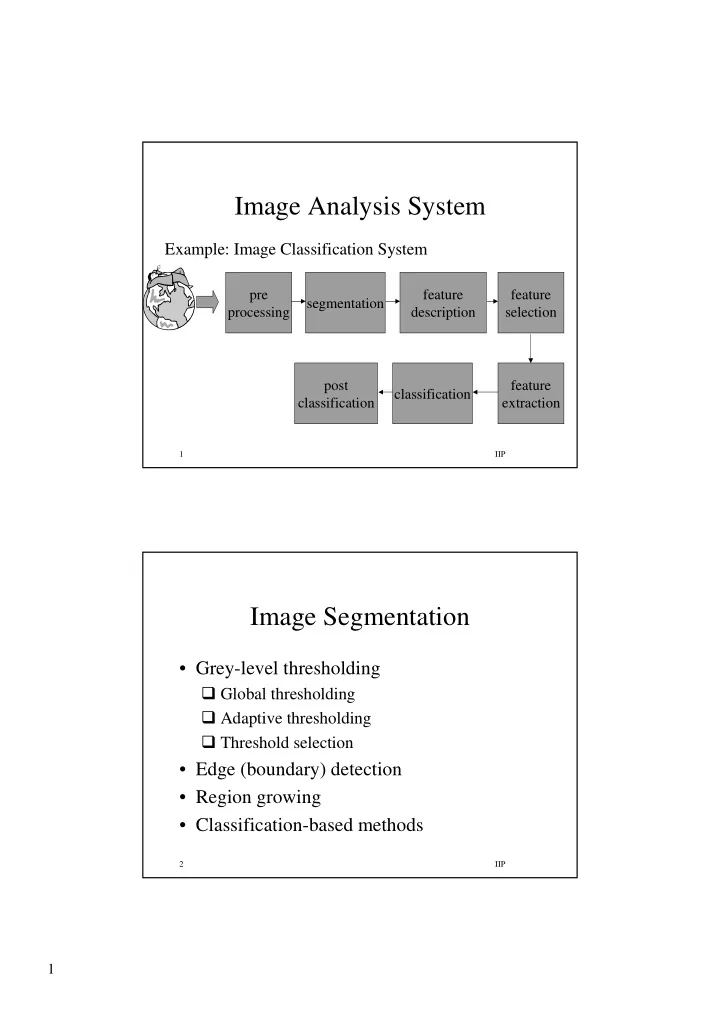
Image Analysis System

classification feature extraction pre processing segmentation feature description feature selection post classification

Example: Image Classification System

IIP 2

Image Segmentation

• Grey-level thresholding

Global thresholding Adaptive thresholding Threshold selection

• Edge (boundary) detection
• Region growing
• Classification-based methods

2

IIP 3

Grey-Level Thresholding (1)

• Global thresholding

   < ≥ = t y x I t y x I y x Ot ) , ( if ) , ( if 1 ) , (    ∈ =

• therwise

) , ( if 1 ) , ( z y x I y x Oz generalized to

IIP 4

Gray-Level Thresholding (2)

• One global

threshold is usually difficult to find

• Other than global

thresholds are sometimes needed

3

IIP 5

Gray-Level Thresholding (3)

• Multiple global

thresholds (via non-linear machine learning)

• Also, adaptive

thresholding (a different threshold for each large region having a bimodal histogram)

• Threshold selection

IIP 6

Edge Detection (1) – Differentiation

• Directional derivative

) 1 , ( ) , ( ) , ( ) , 1 ( ) , ( ) , ( − − = − − = j i f j i f j i f j i f j i f j i f

y x

δ δ in contrast to thresholding extracting characteristic gray level range or some uniformity, edge detection looks for discontinuities in gray level or texture, i.e., border points to be tracked

4

IIP 7

Edge Detection (2) – Laplacian

• 1
• 1

4

• 1
• 1
• 1
• 1
• 1
• 1

8

• 1
• 1
• 1
• 1

Laplacian convolution kernels

) , ( 4 ) 1 , ( ) 1 , ( ) , 1 ( ) , 1 ( ) , (

2

j i f j i f j i f j i f j i f j i f − − + + + − + + = ∇ in a noisy image perform a low-pass filter before the Laplacian

IIP 8

Edge Detection (3) – Template Matching (1)

1

• 1

1

• 1

1

• 1
• 1

1

• 2

2

• 1

1 1 1 1

• 1
• 1
• 1

Prewitt Sobel 1 2 1

• 1
• 2
• 1

Two characteristics: Slope Direction

Prewitt & Sobel are edge operators producing an edge magnitude image that is thresholded

5

IIP 9

Edge Detection (4) – Template Matching (2)

• Sobel operator

IIP 10

Edge Detection (5) – Template Matching (3)

• Other common detectors
• 1
• 1

2

• 1

2

• 1

2

• 1
• 1

line detector (e.g., -45 degrees)

• 3
• 3
• 3

5

• 3

5 5

• 3

Kirsch edge operator line detector finds lines in different orientation Kirsch edge operator responds maximally to an edge oriented in a particular general direction

6

IIP 11

Edge Detection (6) – Boundary Chain Code

Storing segmentation result

Start point + directions (3 bits) Compactness (boundary defines an object) Interior points discarded (not suitable if further processing is necessary)

following edge detection we link edges, generally using thresholding the edges or boundary tracking methods

IIP 12

Region Growing (1)

• Utilises several properties simultaneously
• Suitable for natural scenes where strong a

priori knowledge is not available

• Computationally intensive

divide image into tiny regions (even pixels); define properties in each region (e.g., average gray-level); define boundaries by property values – large difference indicates strong boundary that stands while weak boundary dissolves and regions are merged; repeat for larger regions until no boundaries are weak enough to be dissolved→regions grow and merged until correspond with objects

7

IIP 13

Region Growing (2) – Illustration

Castleman, 1996

IIP 14

Binary Image Processing (IP)

• Morphological image processing (MIP) (a set of

binary IP operations developed from a set- theoretical approach mainly for correcting unsatisfactory initial segmentation)

• Operations can be concatenated producing complex
• perators
• Passing a structuring element (composes of 1’s and

0’s) over the image performing logical operation between the two (similar to convolution)

• Facilitate IP (e.g., pre-processing, computing shape

properties)

8

IIP 15

Logic Operations (pixel-by-pixel)

Gonzalez & Woods, 2002

IIP 16

MIP (1) – Dilation (1)

A boundary point is a pixel that is located inside an object but that has at least one (4 or 8) neighbor outside the object

{ } {

}

{ }

ˆ ˆ | ( ) | ( ) ˆ , sets; | , for

• reflection; - shift

z z

A B z B A z B A A A B B w w b b B z   ⊕ = ∩ ≠ ∅ = ∩ ⊆   = = − ∈

incorporating into the object all the background points that touch it, leaving it larger in area by that amount.

• bjects that are separated by

less than three pixels become connected. useful for filling holes in the segmented objects.

9

IIP 17

MIP (2) – Dilation (2)

Gonzalez & Woods, 2002

note: recall the convolution operation

IIP 18

MIP (3) – Dilation (3)

Gonzalez & Woods, 2002

10

IIP 19

MIP (1) – Erosion (1)

A boundary point is a pixel that is located inside an object but that has at least one (4 or 8) neighbor outside the object

eliminating all the boundary points from an object, leaving the object smaller in area by one pixel all around its perimeter. narrowing to less than 3 pixels thick→disconnection → useful for removing from a segmented image objects that are too small to be of interest.

{ }

| ( )z A B z B A ⊗ = ⊆

IIP 20

MIP (2) – Erosion (2)

Gonzalez & Woods, 2002

11

IIP 21

MIP (3) – Erosion (3)

Gonzalez & Woods, 2002

an example of opening

IIP 22

Morphological IP (2) – Matlab (1)

Matlab IP Toolbox, Mathworks Inc.

12

IIP 23

Morphological IP (3) – Matlab (2)

Matlab IP Toolbox, Mathworks Inc.

IIP 24

Morphological IP (4) – Thinning vs. Skeletonization

thinning skeleton- ization

Castleman, 1996

thinning Thinning – pixels candidates for removal (due to erosion) are removed

• nly if not destroying connectivity

Skeletonization (MAT) – locus of centers of all circles tangent to the boundary at two or more disjoint points

13

IIP 25

Classification-Driven Segmentation (1)

• Avoiding threshold selection
• Modeling of shape or curvature is unnecessary
• Avoiding excessive heuristics
• Example: classification-driven partially
• ccluded object segmentation (CPOOS)

IIP 26

CPOOS (2)

A flow chart of the CPOOS method

Lerner et al., 1998

14

IIP 27

CPOOS (3)

Lerner et al., 1998

application to human chromosome image segmentation

IIP 28

CPOOS (4)

Lerner et al., 1998

different hypotheses

15

IIP 29

CPOOS (5)

Lerner et al., 1998

scoring hypotheses

IIP 30

CPOOS (6)

Lerner et al., 1998

performance evaluation