. . . . . . . . If you want to use a single number to - - PowerPoint PPT Presentation

if you want to use a single number to describe a whole
SMART_READER_LITE
LIVE PREVIEW

. . . . . . . . If you want to use a single number to - - PowerPoint PPT Presentation

Factor Analysis and Beyond Covariance matrix Chris Williams, School of Informatics Let denote an average University of Edinburgh Overview Suppose we have a random vector X = ( X 1 , X 2 , . . . , X d ) T Principal Components


slide-1
SLIDE 1

Factor Analysis and Beyond

Chris Williams, School of Informatics University of Edinburgh

Overview

  • Principal Components Analysis
  • Factor Analysis
  • Independent Components Analysis
  • Non-linear Factor Analysis
  • Reading: Handout on “Factor Analysis and Beyond”, Jordan §14.1

Covariance matrix

  • Let denote an average
  • Suppose we have a random vector X = (X1, X2, . . . , Xd)T
  • X denotes the mean of X, (µ1, µ2, . . . µd)T
  • σii = (Xi − µi)2 is the variance of component i (gives a measure of

the “spread” of component i)

. . . . . . . . . . . . . . . . . . . . . . . . . .

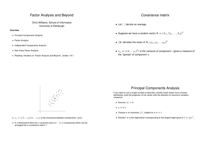
  • σij = (Xi − µi)(Xj − µj) is the covariance between components i and j
  • In d-dimensions there are d variances and d(d − 1)/2 covariances which can be

arranged into a covariance matrix S

Principal Components Analysis

If you want to use a single number to describe a whole vector drawn from a known distribution, pick the projection of the vector onto the direction of maximum variation (variance)

  • Assume x = 0
  • y = w.x
  • Choose w to maximize y2, subject to w.w = 1
  • Solution: w is the eigenvector corresponding to the largest eigenvalue of S = xxT
slide-2
SLIDE 2
  • Generalize this to consider projection from d dimensions down to m
  • S has eigenvalues λ1 ≥ λ2 ≥ . . . λd ≥ 0
  • The directions to choose are the first m eigenvectors of S corresponding to λ1, . . . , λm
  • wi.wj = 0

i = j

  • Fraction of total variation explained by using m principal components is

m

i=1 λi

d

i=1 λi

  • PCA is basically a rotation of the axes in the data space

Factor Analysis

  • A latent variable model; can the observations be explained in terms of a

small number of unobserved latent variables ?

  • FA is a proper statistical model of the data; it explains covariance

between variables rather than variance (cf PCA)

  • FA has a controversial rˆ
  • le in social sciences
  • visible variables : x = (x1, . . . , xp),
  • latent variables: z = (z1, . . . , zm), z ∼ N(0, Im)
  • noise variables: e = (e1, . . . , ep), e ∼ N(0, Ψ), where

Ψ = diag(ψ1, . . . , ψp). Assume x = µ + Wz + e then covariance structure of x is C = WW T + Ψ W is called the factor loadings matrix p(x) is like a multivariate Gaussian pancake p(x|z) ∼ N(Wz + µ, Ψ) p(x) =

  • p(x|z)p(z)dz

p(x) ∼ N(µ, WW T + Ψ)

slide-3
SLIDE 3
  • Rotation of solution: if W is a solution, so is WR where RRT = Im as

(WR)(WR)T = WW T. Causes a problem if we want to interpret

  • factors. Unique solution can be imposed by various conditions, e.g. that

W TΨ−1W is diagonal.

  • Is the FA model a simplification of the covariance structure? S has

p(p + 1)/2 independent entries. Ψ and W together have p + pm free parameters (and uniqueness condition above can reduce this). FA model makes sense if number of free parameters is less than p(p + 1)/2.

FA example

[from Mardia, Kent & Bibby, table 9.4.1]

  • Correlation matrix

mechanics vectors algebra analysis statstics      1 0.553 0.547 0.410 0.389 1 0.610 0.485 0.437 1 0.711 0.665 1 0.607 1     

  • Maximum likelihood FA (impose that W TΨ−1W is diagonal). Require

m ≤ 2 otherwise more free parameters than entries in S.

m = 1 m = 2 (not rotated) m = 2 (rotated) Variable w1 w1 w2 ˜ w1 ˜ w2 1 0.600 0.628 0.372 0.270 0.678 2 0.667 0.696 0.313 0.360 0.673 3 0.917 0.899

  • 0.050

0.743 0.510 4 0.772 0.779

  • 0.201

0.740 0.317 5 0.724 0.728

  • 0.200

0.698 0.286

  • 1-factor and first factor of the 2-factor solutions differ (cf PCA)
  • problem of interpretation due to rotation of factors

FA for visualization

p(z|x) ∝ p(z)p(x|z) Posterior is a Gaussian. If z is low dimensional. Can be used for visualization (as with PCA)

x x

  • = z w

x

1 2

data space z

. .

latent space

slide-4
SLIDE 4

Learning W, Ψ

  • Maximum likelihood solution available (Lawley/J¨
  • reskog).
  • EM algorithm for ML solution (Rubin and Thayer, 1982)

– E-step: for each xi, infer p(z|xi) – M-step: do linear regression from z to x to get W

  • Choice of m difficult (see Bayesian methods later).

Comparing FA and PCA

  • Both are linear methods and model second-order structure S
  • FA is invariant to changes in scaling on the axes, but not rotation invariant

(cf PCA).

  • FA models covariance, PCA models variance

Probabilistic PCA

[Tipping and Bishop (1997)]

Let Ψ = σ2I.

  • In this case WML spans the space defined by the first m eigenvectors of

S

  • PCA and FA give same results as Ψ → 0.

Example Application: Handwritten Digits Recognition

Hinton, Dayan and Revow, IEEE Trans Neural Networks 8(1), 1997

  • Do digit recognition with class-conditional densities
  • 8 × 8 images ⇒ 64 · 65/2 entries in the covariance matrix.
  • 10-dimensional latent space used
  • Visualization of W matrix. Each hidden unit gives rise to a weight image ...
  • In practice use a mixture of FAs!
slide-5
SLIDE 5

Useful Texts

  • n PCA and FA
  • B. S. Everitt and G. Dunn “Applied Multivariate Data Analysis” Edward

Arnold, 1991.

  • C. Chatfield and A. J. Collins “Introduction to Multivariate Analysis”,

Chapman and Hall, 1980.

  • K. V. Mardia, J. T. Kent and J. M. Bibby “Multivariate Analysis”, Academic

Press, 1979.

Independent Components Analysis

  • A non-Gaussian latent variable model, plus linear transformation, e.g.

P(z) ∝

m

  • i=1

e−|zi| x = Wz + µ + e

  • Rotational symmetry in z-space is now broken
  • p(x) is non-Gaussian, go beyond second-order statistics of data for fitting model
  • Can be used with dim(z) = dim(x) for blind source separation
  • http://www.cnl.salk.edu/~tony/ica.html

Non-linear Factor Analysis

P(x) =

  • P(x|z)P(z)dz

For factor analysis

P(x|z) ∼ N(Wz + µ, σ2I)

If we make the prediction of the mean a non-linear function of z, we get non-linear factor analysis, with P(x|z) ∼ N(φ(z), σ2I) and φ(z) = (φ1(z), φ2(z), . . . , φp(z))T. However, there is a problem— we can’t do the integral analytically, so we need to approximate it.

P(x) ≃ 1 K

K

  • k=1

P(x|zk)

where the samples zk are drawn from the density P(z). Note that the approximation to P(x) is a mixture of Gaussians.

slide-6
SLIDE 6

. . . . . . . . .

z z x x x

1 1 2 2 3

φ

  • Generative Topographic Mapping (Bishop, Svensen and Williams, 1997/8)

Fitting the Model to Data

  • Adjust the parameters of φ and σ2 to maximize the log likelihood of the

data.

  • For a simple form of mapping φ(z) =

i wiφi(z) we can obtain EM

updates for the weights {wi} and the variance σ2.

  • We are fitting a constrained mixture of Gaussians to the data. The

algorithm works quite like the SOM (but is more principled as there is an

  • bjective function).

Visualization

  • The mean may be a

bad summary of the posterior distribution. +

z P(z|x)