[PDF] - http://www.stat.sc.edu/~dryden/course/ild-ch-04.pdf Statistical PDF Document

SLIDE 1

Statistical Shape Analysis Ian Dryden (University of Nottingham)

Ian.Dryden@Nottingham.ac.uk http://www.maths.nott.ac.uk/

ild

3e cycle romand de statistique et probabilit´ es appliqu´ es Les Diablerets, Switzerland, March 7-10, 2004.

1

Session I Dryden and Mardia (1998, chapters 1,2,3,4)

✁ Introduction ✁ Motivation and applications ✁ Size and shape coordinates ✁ Shape space ✁ Shape distances.

2

In a wide variety of applications we wish to study the geometrical properties of objects. We wish to measure, describe and compare the size and shapes of objects Shape: location, rotation and scale information (simi- larity transformations) can be removed. [Kendall, 1984] Size-and-shape: location, rotation (rigid body trans- formations) can be removed.

3

An object’s shape is invariant under the similarity trans- formations of translation, scaling and rotation.

Two mouse second thoracic vertebra (T2 bone) out-

lines with the same shape.

4

http://www.stat.sc.edu/~dryden/course/ild-ch-04.pdf

SLIDE 2

From Galileo (1638) illustrating the differences in shapes

f the bones of small and large animals.

5

✁ Landmark: point of correspondence on each object

that matches between and within populations. Different types: anatomical (biological), mathematical, pseudo, quasi

6

T2 mouse vertebra with six mathematical landmarks (line junctions) and 54 pseudo-landmarks.

7

✁ Bookstein (1991)

Type I landmarks (joins of tissues/bones) Type II landmarks (local properties such as maximal curvatures) Type III landmarks (extremal points or constructed land- marks)

✁ Labelled or un-labelled configurations

8

SLIDE 3

F 1 2 3 A 1 2 3 B 2 1 3 D 2 1 3 2 C 1 3 E 2 3 1

Six labelled triangles: A, B have the same size and shape; C has the same shape as A, B (but larger size); D has a different shape but its labels can be permuted to give the same shape as A, B, C; triangle E can be reflected to have the same shape as D; triangle F has a different shape from A,B,C,D,E.

9

Traditional methods

ratios of distances between landmarks or angles sub-

mitted to multivariate analysis

the full geometry usually if often lost
collinear points?
interpretation of shape differences in multivariate space?

10

Geometrical shape analysis Rather than working with quantities derived from or- ganisms one works with the complete geometrical ob- ject itself (up to similarity transformations). In the spirit of D’Arcy Thompson (1917) who consid- ered the geometric transformations of one species to another We conside a shape space obtained directly from the landmark coordinates, which retains the geometry of a point configuration at all stages.

11

✁ Pioneers: Fred Bookstein and David Kendall

Summaries of the field are given by Bookstein (1991, Cambridge), Small (1996, Springer), Dryden and Mar- dia (1998, Wiley), Kendall et al (1999, Wiley), Lele and Richstmeier (2001, Chapman and Hall).

12

SLIDE 4

MR brain scan

13

The map of 52 megalithic sites (+) that form the ‘Old Stones of Land’s End’ in Cornwall (from Stoyan et al., 1995).

14

0.4
0.2

0.0 0.2 0.4

0.4
0.2

0.0 0.2 0.4 1 2 3 4 5 6 7 8 9 10 11 12 13

Handwritten digit 3

15 pr ba

l

b n na st Face Braincase

Ape cranium

16

SLIDE 5

(a) (b)

Electrophoretic gel matching

17

50 100 150 200 250 50 100 150 200

✂

250 S S S S S S S S S

Face recognition

18

Proton density weighted MR image

19

Cortical surface extracted from MR scan

20

SLIDE 6

203 Pseudo-landmarks on the cortical surface of the brain

21

OUR FOCUS:

✄

landmarks in

☎

real dimensions

✆

is a

✄ ✝ ☎

matrix (

✞ ✟ ✠ ✡ ☛ ☞ ✌ ✍ ✎ ✏ ✑ ✍ ✏ ✒ ✓ ✑ ✍ ✓ ✔ ✓ ✕

) Invariance with respect to Euclidean similarity group (translation, scale and rotation) =

✖ ✠ ✡ ☞ ✝ ✠ ✡ ✗ ✝ ✘ ✙ ✚ ☎ ✛ ✜

Size.... Any positive real valued function

✢ ✚ ✆ ✛ such that ✢ ✚ ✣ ✆ ✛ ✟ ✣ ✢ ✚ ✆ ✛ for a positive scalar ✣ .

22

✁ Centroid size: ✘ ✚ ✆ ✛ ✟ ✤ ✥ ✆ ✤ ✟ ✦ ☛ ✧ ★ ✩ ✪ ☞ ✧ ✫ ✩ ✪ ✚ ✆ ★ ✫ ✬ ✭ ✆ ✫ ✛ ✮

where

✭ ✆ ✫ ✟ ✪ ☛ ✯ ☛ ★ ✩ ✪ ✆ ★ ✫ and ✥ ✟ ✰ ☛ ✬ ✱ ✄ ✱ ☛ ✱ ✲ ☛ ✤ ✆ ✤ ✟ ✦ ✕ ✳ ✴ ✍ ✓ ✚ ✆ ✲ ✆ ✛ - Euclidean norm, ✰ ☛ - ✄ ✝ ✄ identity matrix, ✱ ☛ - ✄ ✝ ✱ vector of ones.

23

An alternative size measure is the baseline size, i.e. the length between landmarks 1 and 2:

✵ ✪ ✮ ✚ ✆ ✛ ✟ ✤ ✚ ✆ ✛ ✮ ✬ ✚ ✆ ✛ ✪ ✤ ✶

This was used as early as 1907 by Galton for normal- izing faces. Other size measures: square root of area, cube root

f volume

24

SLIDE 7

Shape coordinates: Fixed coordinate system vs Local Coordinate system Are angles appropriate.....??

1 2 3 1 2 3 1 2 3

25

Landmarks:

✷ ✪ ✸ ✷ ✮ ✸ ✶ ✶ ✶ ✸ ✷ ☛ ✹ ✺ ✁

Bookstein shape coordinates (1984,1986) (For two dimensional data)

Re(z)

Im(z)

200 -100

100 200

200 -100

100 200

✻

Re(z)

Im(z)

200 -100

100 200

200 -100

100 200

✻

Re(z)

Im(z)

200 -100

100 200

200 -100

100 200

Re(z)

Im(z)

0.5

0.0 0.5

0.5

0.0 0.5 1.0

Shape:

✼ ✽ ✫ ✟ ✾ ✿ ❀ ✾ ❁ ✾ ❂ ❀ ✾ ❁ ✬ ❃ ✶ ❄ ✸ ✚ ❅ ✟ ❆ ✸ ✶ ✶ ✶ ✸ ✄ ✛

26

(a)
20 -10

10 20

20 -10

10 20 1 2 3

(b)
20 -10

10 20

20 -10

10 20 1 2 3

(c)
20 -10

10 20

20 -10

10 20 1 2 3

(d)
0.5

0.0 0.5

0.5

0.0 0.5 1.0 1 2 3

In real co-ordinates:

❇ ❈ ❉ ✩ ❀ ✪ ✮ ✗ ❊ ❋ ✾

❀

✾ ❍ ■ ❋ ✾ ❉ ❀ ✾ ❍ ■ ✗ ❋ ❏

❀

❏ ❍ ■ ❋ ❏ ❉ ❀ ❏ ❍ ■ ❑ ▲ ▼

❍
◆

❖ ❈ ❉ ✩ ❊ ❋ ✾

❀

✾ ❍ ■ ❋ ❏ ❉ ❀ ❏ ❍ ■ ❀ ❋ ❏

❀

❏ ❍ ■ ❋ ✾ ❉ ❀ ✾ ❍ ■ ❑ ▲ ▼

❍
◆

where

✫ ✩ P ◆ ◗ ◗ ◗ ◆ ☛

,

▼

❍
✩

❋ ✾

❀

✾ ❍ ■

✗

❋ ❏

❀

❏ ❍ ■

❘

❙

and

❀ ❚ ❯ ❇ ❈ ❉ ◆ ❖ ❈ ❉ ❯ ❚

.

27

The outline of a microfossil with three landmarks (from Bookstein, 1986).

28

SLIDE 8

U

V

❱

0.2 0.3 0.4 0.5 0.6 0.4 0.5 0.6 0.7 0.8 60 65 64 65 67 71 72 71 74 75 76 84 84 84 87 88 88 88 92 100 100

A scatter plot of (U+1/2) for the Bookstein shape vari- ables for some microfossil data. (Bookstein, 1986)

29

slog

0.32

❲

0.36 0.40 0.44

•
•
8.2

8.4 8.6 8.8 9.0

❳

9.2

•
0.32

❨

0.36 0.40 0.44

•
U
•
8.2

8.4 8.6 8.8 9.0 9.2

•
0.45

❲

0.55 0.65 0.75

❲

0.45 0.55 0.65 0.75

V

30

u

❩

v

0.5

0.0

❬

0.5

❬

0.5

0.0 0.5 1

❭

2

❪

6

❫

3

❴

5

❵

4

❛

A scatter plot of the Bookstein shape variables for the T2 mouse data.

31

B

❜

U

❝

VB

2
1

❬

1

❭

2

❪

2
1

1 2 E

❞

F

❡

A

❢

B

❜

O

❣

The shape space of triangles, using Bookstein’s co-

rdinates

✚ ❤ ✽ ✸ ✐ ✽ ✛ . All triangles could be relabelled

and reflected to lie in the shaded region.

32

SLIDE 9

Kendall’s shape coordinates Remove location

❥ ❦ ✟ ❧ ❥ ♠ ✟ ✚ ❥ ✪ ✸ ✶ ✶ ✶ ✸ ❥ ☛ ❀ ✪ ✛ ✲ ✼ ♥ ✫ ♦ ♣ q ♥ ✫ ✟ ❥ ✫ ❀ ✪ ❥ ✪ ✚ ❅ ✟ ❆ ✸ ✶ ✶ ✶ ✸ ✄ ✛ ✶

Simple 1-1 linear correspondence with Booklstein S.V. (equ. 2.11 of book) For triangles Kendall’s SV sends baseline to

✬ ✱ r ✦ ❆ ✸ ✱ r ✦ ❆

33

✁ Kendall’s shape sphere (1983) (triangles only)

Flat triangles

1 2 3 1 2 3

Isosceles triangles Equilateral (North pole) Reflected equilateral (South pole) (Equator)

Right-angled

Unlabelled

φ=0 φ=π/3 φ=5π/3 φ=2π/3 θ=π/2 θ=0 θ=π

A mapping from Kendall’s shape variables to the sphere is

✷ ✟ ✱ ✬ s ✮ t ✚ ✱ ♦ s ✮ ✛ ✸ ✉ ✟ ✼ ♥ P ✱ ♦ s ✮ ✸ ❥ ✟ q ♥ P ✱ ♦ s ✮

and

s ✮ ✟ ✚ ✼ ♥ P ✛ ✮ ♦ ✚ q ♥ P ✛ ✮ , so that ✷ ✮ ♦ ✉ ✮ ♦ ❥ ✮ ✟ ✪ ✈ .

34

Kendall’s spherical shape shape variables

✚ ✇ ✸ ① ✛ are

then given by the usual polar coordinates

✷ ✟ ✱ t ✔ ✏ ✑ ✇ ✍ ✎ ✔ ① ✸ ✉ ✟ ✱ t ✔ ✏ ✑ ✇ ✔ ✏ ✑ ① ✸ ❥ ✟ ✱ t ✍ ✎ ✔ ✇ ✸

where

❃ ② ✇ ② ③

is the angle of latitude and

❃ ② ① ④ t ③

is the angle of longitude.

35

Kendall’s Bell

36

SLIDE 10

The Schmidt net for 1/12 sphere

⑤ ✟ t ✔ ✏ ✑ ⑥ ✇ t ⑦ ✸ ⑧ ✟ ① ⑨ ❃ ② ⑤ ② ✦ t ✸ ❃ ② ⑧ ④ t ③ ✶

0.5

0.0 0.5

1.5
1.0
0.5

0.0

A

B C

A

B C

A

B C

A

B C

A

B C • A B C

A

B C

A

B C

A

B C

A

B C

A

B C

A

B C

A

B C

A

B C

A

B C

A

B C

A

B C

A

B C

A

B C

A

B C

A

B C

A

B C

A

B C

A

B C

A

B C

A

B C

A

B C

A

B C

A

B C

A

B C

A

B C

A

B C

A

B C

A

B C

A

B C

A

B C

A

B C

37

Bookstein coordinates - 3D Landmarks

✆ ★ ✟ ✚ ✷ ✪ ★ ✸ ✷ ✮ ★ ✸ ✷ P ★ ✛ ✲ ✼ ✫ ✟ ✚ ✼ ✪ ✫ ✸ ✼ ✮ ✫ ✸ ✼ P ✫ ✛ ✲ ✟ ✱ ✤ ✆ ✮ ✬ ✆ ✪ ✤ ⑩ ❶ ✆ ✫ ✬ ✚ ✆ ✪ ♦ ✆ ✮ ✛ t ❷ ✸ ❅ ✟ ❆ ✸ ✶ ✶ ✸ ✄

where

⑩

is a

❆ ✝ ❆

rotation matrix (a function of

✚ ✆ ✪ ✸ ✆ ✮ ✸ ✆ P ✛ ) and ✆ ✪ ❸ ✚ ✬ ✱ r t ✸ ❃ ✸ ❃ ✛ ✲ ✸ ✆ ✮ ❸ ✚ ✱ r t ✸ ❃ ✸ ❃ ✛ ✲ ✸ ✆ P ❸ ✼ P ✟ ✚ ✼ ✪ P ✸ ✼ ✮ P ✸ ❃ ✛ ✲

where

✼ ✮ P ❹ ❃ , ✼ P P ✟ ❃

and

✆ ✫ ❸ ✼ ✫

for

❅ ✟ ❺ ✸ ✶ ✶ ✶ ✸ ✄ .

38

(a) (b)

Bookstein 3D coordinates

39

Goodall-Mardia QR shape coordinates

❹ t

D Helmertized landmarks

✆ ❦ ✟ ❧ ✆

(

✄ ✝ ☎

matrix) SIZE AND SHAPE (JOINTLY)

✆ ❦ ✟ ❻ ❼ ✸ ❼ ✹ ✘ ✙ ✚ ☎ ✛ ✸ ❻

is lower triangular SHAPE:

❽ ✟ ❻ r ✤ ❻ ✤

40

SLIDE 11

Shape coordinates

1. FILTER OUT TRANSLATION:

a) Shift centroid to origin b) Take linear orthogonal contrasts, e.g. Helmert con- trasts c) Shift baseline midpoint to origin

2. RE-SCALE:

a) Re-scale to unit centroid size b) Re-scale to unit area c) Re-scale to a standard baseline length d) Re-scale to minimize ‘distance’ to a template

3. REMOVE ROTATION:

a) Rotate baseline to horizontal b) Rotate to minimize ‘distance’ to a template Bookstein shape coordinates: 1c/2c/3a Kendall shape coordinates: 1b/2c/3a Procrustes shape coordinates: 1a/2d/3b

41

SHAPE SPACE....Kendall (1984)

1. Remove location (Pre-multiply by Helmert sub-matrix)

✆ ❦ ✟ ❧ ✆

where

❅ th row of the Helmert sub-matrix ❧

is given by,

✚ ❾ ✫ ✸ ✶ ✶ ✶ ✸ ❾ ✫ ✸ ✬ ❅ ❾ ✫ ✸ ❃ ✸ ✶ ✶ ✶ ✸ ❃ ✛ ✸ ❾ ✫ ✟ ✬ ✖ ❅ ✚ ❅ ♦ ✱ ✛ ✜ ❀ ❁ ❂

and the

❾ ✫

is repeated

❅

times and zero is repeated

✄ ✬ ❅ ✬ ✱ times, ❅ ✟ ✱ ✸ ✶ ✶ ✶ ✸ ✄ ✬ ✱ .

Note

✥ ✟ ❧ ✲ ❧

(centering matrix) so

✤ ✆ ❿ ✤ ✟ ✤ ✆ ❦ ✤ ✟ ✘ ✚ ✆ ✛ ✶ (centroid size)

42

2. Remove size (rescale)

➀ ✟ ✆ ❦ ✘ ✚ ✆ ✛ ✟ ❧ ✆ ✤ ❧ ✆ ✤ ✶ ✁ ➀

is the PRESHAPE (

✹ ✘ ❋ ☛ ❀ ✪ ■ ☞ ❀ ✪

)

3. Remove rotation

➁ ✆ ➂ ✟ ✖ ➀ ❼ ➃ ❼ ✹ ✘ ✙ ✚ ☎ ✛ ✜ ✸ ✁ ➁ ✆ ➂ is the SHAPE of ✆

.

43

✁ Dimensions....

Original configuration:

✄ ✝ ☎

Centered configuration:

✄ ☎ ✬ ☎

Preshape:

✄ ☎ ✬ ☎ ✬ ✱

Shape:

✄ ☎ ✬ ☎ ✬ ✱ ✬ ☎ ✚ ☎ ✬ ✱ ✛ r t ✁ Shape space is non-Euclidean

44

SLIDE 12

SHAPE SPACES Assume

✄ ❹ ☎ ♦ ✱ . [ ✄ points in ☎

Euclidean dimen- sions]

☎ ✟ ✱ : ➄ ☛ ✪ is a unit radius ✚ ✄ ✬ t ✛ -sphere. ☎ ✟ t : ➄ ☛ ✮ is the complex projective space ✺ ➅ ☛ ❀ ✮ . ☎ ➆ t : ➄ ☛ ☞

has a singularity set

③ ✚ ➇ ☞ ❀ ✮ ✛ of dimen-

sion

☎ ✬ t

and is NOT a homogeneous space. For

☎ ➆ t

the space spaces

➄ ☞ ✗ ✪ ☞

are topological spheres.

45 Write

➈ ✩ ➉ ➊ ➋ ◆ ❙ ➌ ➍ , for the pseudo-singular value decom-

position where

➉ ➎ ➏ ➐ ❋ ☞ ❀ ✪ ■ ◆ ➍ ➎ ➏ ➐ ❋ ☛ ❀ ✪ ■ , and ➋ ✩ ➑ ➒ ➓ ➔ ❋ → ❍ ◆ ◗ ◗ ◗ ◆ → ➣ ■ . Let ↔ ↕ ➣ ✩ ➙ ❊ ➈ ➎ ➏ ↕ ➣ ➛ → ❍ ❘ ◗ ◗ ◗ ❘ → ➣ ➜ ❍ ❘ ➝ → ➣ ➝ ❑ ➒ ➞ ☛ ✩ ☞ ✗ ✪ ❊ ➈ ➎ ➏ ↕ ➣ ➛ → ❍ ❘ ◗ ◗ ◗ ❘ → ➣ ➜ ❍ ❘ → ➣ ❑ ➒ ➞ ☛ ❘ ☞ ✗ ✪

Le and DG Kendall (1993, Annals of Statistics) Theorem On

➟ ❋ ↔ ↕ ➣ ■ , the Riemannian metric can be expressed

as

➠ ➡

✩

➣ ✧ ➢ ➤

➠

→

➢

✗ ❶ ➣ ✧ ➢ ➤

→

➢ → ❍ ➠ → ➢ ❷

✗

✧ ❍ ➥ ➢ ➦ ❉ ➥ ➣ ❋ →

➢

❀ →

❉

■

→
➢

✗ →

❉

➧

➢

❉ ✗ ➣ ✧➢ ➤ ❍ ↕ ➜ ❍ ✧ ❉ ➤ ➣ ➨ ❍ →

➢

➧

➢

❉ ◆

where

➧ ➢ ❉ are co-ordinates for ➏ ➐ ❋ ☛ ❀ ✪ ■ .

46

Planar case:

☎ ✟ t

dimensional data

➄ ☛ ☞ ✟ ✘ ☛ ✮ r ✘ ✙ ✚ t ✛ ✟ ✺ ➅ ☛ ❀ ✮

Helmertized landmarks

❥ ❦ ✟ ❧ ❥ ♠ ✟ ✚ ❥ ✪ ✸ ✶ ✶ ✶ ✸ ❥ ☛ ❀ ✪ ✛ ✲ ✹ ✺ ☛ ❀ ✪ ✌ ✖ ❃ ✜

Now multiplying by

➩ ✟ s ✓ ★ ➫ ✸ ✚ s ✹ ✠ ✡ ✗ ✸ ➭ ✹ ➁ ❃ ✸ t ③ ✛ ✛

rotates and rescales

❥ ❦ . So, ✖ ➩ ❥ ❦ ➃ ➩ ✹ ✺ ✌ ✖ ❃ ✜ ✜ ✸

is the set representing the SHAPE of

❥ ♠ . This is a

complex line through the origin (but not including it) in

✄ ✬ ✱

dimensions. The union of all such sets is the

complex projective space

✺ ➅ ☛ ❀ ✮

NB:

✺ ➅ ☛ ❀ ✮ ➯ ✘ ✮

47

PLANAR CASE: Procrustes/Riemannian distance Complex configurations

❥ ♠ ✟ ✚ ❥ ♠ ✪ ✸ ✶ ✶ ✶ ✸ ❥ ♠ ☛ ✛ ✲ ✸ ➲ ♠ ✟ ✚ ➲ ♠ ✪ ✸ ✶ ✶ ✶ ✸ ➲ ♠ ☛ ✛ ✲

with centroids

❥ ➳ ✸ ➲ ➳ .

Shape distance

➵ ✚ ❥ ♠ ✸ ➲ ♠ ✛ satisfies ✍ ✎ ✔ ➵ ✚ ❥ ♠ ✸ ➲ ♠ ✛ ✟ ➸ ✯ ☛ ★ ✩ ✪ ✚ ❥ ♠ ★ ✬ ❥ ➳ ✛ ✚ ➲ ♠ ★ ✬ ➲ ➳ ✛ ➸ ✦ ✯ ✤ ❥ ♠ ★ ✬ ❥ ➳ ✤ ✮ ✦ ✯ ✤ ➲ ♠ ★ ✬ ➲ ➳ ✤ ✮

where

➲ ♠ ★ means the complex conjugate of ➲ ♠ ★ .

NB

✍ ✎ ✔ ➵

is the modulus of the complex correlation between

❥ ♠ and ➲ ♠ . ✁ ✄ ✟ ❆ : ➵

is the great circle distance on

✘ ✮ ✚ ✱ r t ✛ .

48

SLIDE 13

Complex configurations

❥ ♠ ✟ ✚ ❥ ♠ ✪ ✸ ✶ ✶ ✶ ✸ ❥ ♠ ☛ ✛ ✲

Bookstein co-ordinates:

➲ ✽ ✫ ✟ ❥ ♠ ✫ ✬ ❥ ♠ ✪ ❥ ♠ ✮ ✬ ❥ ♠ ✪ ✬ ❃ ✶ ❄ ✸ ✚ ❅ ✟ ❆ ✸ ✶ ✶ ✶ ✸ ✄ ✛

Kendall co-ordinates:

➲ ♥ ✫ ✟ ❥ ✫ ❀ ✪ r ❥ ✫ ✸ ✚ ❅ ✟ ❆ ✸ ✶ ✶ ✶ ✸ ✄ ✛

where

✚ ❥ ✪ ✸ ✶ ✶ ✶ ✸ ❥ ☛ ❀ ✪ ✛ ✲ ✟ ❧ ❥ ♠ ✁ Linear relationship: ➺ ♥ ✟ ✦ t ❧ ✪ ➺ ✽

where

❧ ✪ is lower right ✚ ✄ ✬ t ✛ ✝ ✚ ✄ ✬ t ✛ partition of ❧

. For

✄ ✟ ❆ : ➲ ✽ P ✟ ✚ ✦ ❆ r t ✛ ➲ ♥ P

.

49

Session II

✁ Procrustes analysis ✁ Tangent coordinates ✁ Shape variability ✁ Shape models ✁ Tangent space inference ✁ Shapes package.

50

PROCRUSTES ANAL YSIS Juvenile (———) Adult (- - - - - -)

x

y

2000
1000

1000 2000 3000

2000
1000

1000 2000 3000

x

y

2000
1000

1000 2000 3000

2000
1000

1000 2000 3000

Register adult onto juvenile

51

PLANAR PROCRUSTES ANAL YSIS Two centred configurations

✉ ✟ ✚ ✉ ✪ ✸ ✶ ✶ ✶ ✸ ✉ ☛ ✛ ➻

and

➲ ✟ ✚ ➲ ✪ ✸ ✶ ✶ ✶ ✸ ➲ ☛ ✛ ➻ , both in ✺ ☛

, with

✉ ➼ ✱ ☛ ✟ ❃ ✟ ➲ ➼ ✱ ☛ ,

[

✉ ➼ - transpose of the complex conjugate of ✉ ]

Match

➲

nto

✉

using complex linear regression

✉ ✟ ✚ ✣ ♦ ♣ ➽ ✛ ✱ ☛ ♦ ➾ ✓ ★ ➚ ➲ ♦ ➪ ✟ ➁ ✱ ☛ ✸ ➲ ➂ ⑩ ♦ ➪ ✟ ✆ ▼ ⑩ ♦ ➪ ✸ ✆ ▼ ✟ ➁ ✱ ☛ ✸ ➲ ➂ - ‘design’ matrix ⑩ ✟ ✚ ✣ ♦ ♣ ➽ ✸ ➾ ✓ ★ ➚ ✛ ➻

similarity transformation pa-

rameters

52

SLIDE 14

Procrustes match = least squares Minimize the sum of square errors

✵ ✮ ✚ ✉ ✸ ➲ ✛ ✟ ➪ ➼ ➪ ✟ ✚ ✉ ✬ ✆ ▼ ⑩ ✛ ➼ ✚ ✉ ✬ ✆ ▼ ⑩ ✛ ✶

Full Procrustes fit (superimposition) of

➲

n

✉ ➲ ➶ ✟ ✆ ▼ ➹ ⑩ ✟ ✚ ➹ ✣ ♦ ♣ ➹ ➽ ✛ ✱ ☛ ♦ ➹ ➾ ✓ ★ ➘ ➚ ➲ ✸

where

➹ ⑩ ✟ ✚ ✆ ➼ ▼ ✆ ▼ ✛ ❀ ✪ ✆ ➼ ▼ ✉ ,

i.e.

➹ ✣ ♦ ♣ ➹ ➽ ✟ ❃ ✸ ➹ ✇ ✟ ✴ ✳ ➴ ✚ ➲ ➼ ✉ ✛ ✟ ✬ ✴ ✳ ➴ ✚ ✉ ➼ ➲ ✛ ✸ ➹ ➾ ✟ ✚ ➲ ➼ ✉ ✉ ➼ ➲ ✛ ✪ ▲ ✮ r ✚ ➲ ➼ ➲ ✛ ✶

53

Procrustes fit

➲ ➶ ✟ ➲ ➼ ✉ ➲ r ✚ ➲ ➼ ➲ ✛

Procrustes residual vector

s ✟ ✉ ✬ ➲ ➶

Minimized objective function

✵ ✮ ✚ s ✸ ❃ ✛ ✟ ✉ ➼ ✉ ✬ ✚ ✉ ➼ ➲ ➲ ➼ ✉ ✛ r ✚ ➲ ➼ ➲ ✛

(not symmetric unless

✉ ➼ ✉ ✟ ➲ ➼ ➲ )

Initially standardize to unit centroid size.... Full Procrustes distance:

➷ ➬ ✚ ➲ ✸ ✉ ✛ ✟ ✏ ✑ ➮ ➱ ◆ ➚ ◆ ✃ ◆ ❐ ❒ ❒ ❒ ❒ ❒ ✉ ✤ ✉ ✤ ✬ ➲ ✤ ➲ ✤ ➾ ✓ ★ ➚ ✬ ✣ ✬ ♣ ➽ ❒ ❒ ❒ ❒ ❒ ✟ ❮ ✱ ✬ ✉ ➼ ➲ ➲ ➼ ✉ ➲ ➼ ➲ ✉ ➼ ✉ ❰ ✪ ▲ ✮ ✶

54

FULL Procrustes distance

➷ ➬

full set of similarity

transformations used in matching PARTIAL Procrustes distance

➷ ➶

matching over trans-

lation and rotation ONLY For fairly similar shapes they are very similar, as

➷ ➬ ✟ ➷ ➶ ♦ ✙ ✚ ➷ P ➶ ✛ ✟ ➵ ♦ ✙ ✚ ➵ P ✛

In this course for simplicity we shall concentrate on FULL Procrustes matching.

55 1 1 ρ ρ/2

F

/2

P

d d

Section of the pre-shape sphere

56

SLIDE 15

1/2 1/2 ρ dF d/2 ρ

Section of the SHAPE SPHERE FOR TRIANGLES, illustrating the relationship between

➷ ➬ , ➷ ➶

and

➵

57

Procrustes residuals from the match of

➲

nto

✉

are different from

✉ onto ➲

x

y

2000
1000

1000 2000 3000

2000
1000

1000 2000 3000

JUV to ADULT (above):

➹ ✇ ✟ ❺ ❄ ✶ ❄ Ï , ➹ ➾ ✟ ✱ ✶ ✱ ❆ ✱ .

ADULT to JUV:

➹ ✇ Ð ✟ ✬ ❺ ❄ ✶ ❄ Ï , ➹ ➾ Ð ✟ ❃ ✶ Ñ Ò ❄ Ó ✟ ✱ r ✱ ✶ ✱ ❆ ✱

58

Female (left) and Male (right) gorilla skulls

x (a) y

300
200
100

100

100

100 200 x (b) y

300
200
100

100

100

100 200

Mean shape? Shape variance/covariance?

59

CONFIGURATION MODEL Random sample of

Ô

configurations

➲ ✪ ✸ ✶ ✶ ✶ ✸ ➲ Õ

from the perturbation model

➲ ★ ✟ Ö ★ ✱ ☛ ♦ ➾ ★ ✓ ★ ➚ × ✚ Ø ♦ ➪ ★ ✛ ✸ ♣ ✟ ✱ ✸ ✶ ✶ ✶ ✸ Ô ✸

where

Ö ★ ✹ ✺

translations

➾ ★ ✹ ✠ ✡ ✗

scales

❃ ② ✇ ★ ④ t ③

rotations

➪ ★ ✹ ✺

are independent zero mean complex random errors

Ø

is the population mean configuration. AIM: to estimate

➁ Ø ➂ - the shape of Ø

Procrustes mean:

➁ ➹ Ø ➂ ✟ ✴ ✳ ➴ ✏ ✑ ➮ Ù Õ ✧ ★ ✩ ✪ ➷ ✮ ➬ ✚ ➲ ★ ✸ Ø ✛ ✶

60

SLIDE 16

Consider

➲ ★ to be centred: ➲ ✲ ★ ✱ ☛ ✟ ❃ .

(Kent, 1994) Procrustes mean shape

➁ ➹ Ø ➂ is the dom-

inant eigenvector of

✘ ✟ Õ ✧ ★ ✩ ✪ ➲ ★ ➲ ➼ ★ r ✚ ➲ ➼ ★ ➲ ★ ✛ ✟ Õ ✧ ★ ✩ ✪ ❥ ★ ❥ ➼ ★ ✸

where the

❥ ★ ✟ ➲ ★ r ✤ ➲ ★ ✤ ✸ ♣ ✟ ✱ ✸ ✶ ✶ ✶ ✸ Ô , are the pre-

shapes. Proof We wish to minimize

Õ ✧ ★ ✩ ✪ ➷ ✮ ➬ ✚ ➲ ★ ✸ Ø ✛ ✟ Õ ✧ ★ ✩ ✪ ❮ ✱ ✬ Ø ➼ ➲ ★ ➲ ➼ ★ Ø ➲ ➼ ★ ➲ ★ Ø ➼ Ø ❰ ✟ Ô ✬ Ø ➼ ✘ Ø r ✚ Ø ➼ Ø ✛ ✶

Therefore,

➹ Ø ✟ ✴ ✳ ➴ ✔ Ú Û Ü Ù Ü ✩ ✪ Ø ➼ ✘ Ø ✶

Hence, result follows.

61

✁ Procrustes fits: match ➲ ★ to ➹ Ø ➲ ➶ ★ ✟ ➲ ➼ ★ ➹ Ø ➲ ★ r ✚ ➲ ➼ ★ ➲ ★ ✛ ✸ ♣ ✟ ✱ ✸ ✶ ✶ ✶ ✸ Ô ✸

NB Arithmetic mean:

✪ Õ ✯ Õ ★ ✩ ✪ ➲ ➶ ★

has same shape as

➹ Ø . ✁ Procrustes residuals s ★ ✟ ➲ ➶ ★ ✬ ÝÞ ✱ Ô Õ ✧ ★ ✩ ✪ ➲ ➶ ★ ßà ✸ ♣ ✟ ✱ ✸ ✶ ✶ ✶ ✸ Ô ✸

62

Procrustes fits (Generalized Procrustes analysis)

0.6
0.4
0.2

0.0 0.2 0.4 0.6

0.6
0.4
0.2

0.0 0.2 0.4 0.6

Female gorillas

63

0.6
0.4
0.2

0.0 0.2 0.4 0.6

0.6
0.4
0.2

0.0 0.2 0.4 0.6

Male Gorillas

SLIDE 17

x y

150
100
50

50 100 150

150
100
50

50 100 150

The male (—-) and female (- - -) full Procrustes mean shapes registered by GPA.

64

Other mean shape estimates:

✁ Bookstein mean shape

Take sample mean of Bookstein coordinates

❤ ✽

u

v

á

1.0
0.5

0.0 0.5 1.0

1.0
0.5

0.0 0.5 1.0 7 4 1 2 3 5 6 8

â

1 2 3 5 6 8

â

1 2

ã

3

ä

5

å

6 8 1 2

ã

3 5

å

6 8

â

1 2 3 5

å

6 8 1 2 3

ä

5 6 8

â

1 2 3 5 6 8 1 2

ã

3 5 6 8 1 2

ã

3 5 6 8

â

1 2

ã

3 5

å

6 8 1 2

ã

3 5 6 8 1 2 3 5 6 8 1 2 3

ä

5 6 8 1 2

ã

3

ä

5

å

6 8 1 2 3 5 6 8 1 2 3 5 6 8 1 2 3 5 6 8 1 2 3

ä

5 6 8 1 2 3 5 6 8

â

1 2 3 5 6 8 1 2 3 5 6 8 1 2

ã

3

ä

5 6 8 1 2 3 5

å

6 8 1 2 3 5 6 8 1 2 3 5 6 8 1 2 3 5 6 8 1 2 3 5

å

6 8 1 2 3 5 6 8

â

1 2

ã

3 5 6 8 1 2 3 5 6 8

â

Female Gorillas

65

u

v

1.0
0.5

0.0 0.5 1.0

1.0
0.5

0.0 0.5 1.0 7 4 1 2 3 5 6 8 1 2 3 5 6 8 1 2 3 5 6 8 1 2 3 5 6 8 1 2 3 5 6 8 1 2 3 5 6 8 1 2 3 5 6 8 1 2 3 5 6 8 1 2 3 5 6 8 1 2 3 5 6 8 1 2 3 5 6 8 1 2 3 5 6 8 1 2 3 5 6 8 1 2 3 5 6 8 1 2 3 5 6 8 1 2 3 5 6 8 1 2 3 5 6 8 1 2 3 5 6 8 1 2 3 5 6 8 1 2 3 5 6 8 1 2 3 5 6 8 1 2 3 5 6 8 1 2 3 5 6 8 1 2 3 5 6 8 1 2 3 5 6 8 1 2 3 5 6 8 1 2 3 5 6 8 1 2 3 5 6 8 1 2 3 5 6 8

Male Gorillas

66

[In Book chapter 12]

✁ MDS mean shape (Kent, 1994; Lele 1991)

Obtain average squared Euclidean distance matrix

✵

let

æ ✟ ✬ ✪ ✮ ✥ ✵ ✥

(centred inner product matrix) Let

ç ✪ ✸ ✶ ✶ ✶ ✸ ç è be the scaled eigenvectors ✞ ✵ ✘ ☞ ✚ ✵ ✛ ✟ ➁ ç ✪ ✸ ç ✮ ✸ ✶ ✶ ✶ ✸ ç ☞ ➂

(invariant under reflections too)

✁

IMPORTANT: If shape variations small the mean shape estimates are approximately linearly related. i.e. Multivariate normal based inference will be equiv- alent to first order. (Kent, 1994)

67

SLIDE 18

Tangent coordinates Consider complex landmarks

❥ ♠ ✟ ✚ ❥ ♠ ✪ ✸ ✶ ✶ ✶ ✸ ❥ ♠ ☛ ✛ ➻

with pre-shape

❥ ✟ ✚ ❥ ✪ ✸ ✶ ✶ ✶ ✸ ❥ ☛ ❀ ✪ ✛ ➻ ✟ ❧ ❥ ♠ r ✤ ❧ ❥ ♠ ✤ ✶

Let

Ö

be a complex pole on the complex pre-shape sphere usually chosen as an average shape. Let us rotate the configuration by an angle

✇ to be as

close as possible to the pole and then project onto the tangent plane at

Ö , denoted by ❻ ✚ Ö ✛ . Note that ➹ ✇ ✟ ✴ ✳ ➴ ✚ ✬ Ö ➼ ❥ ✛ minimizes ✤ Ö ✬ ❥ ✓ ★ ➚ ✤ ✮ .

68

The partial Procrustes tangent coordinates for a planar shape are given by

q ✟ ✓ ★ ➘ ➚ ➁ ✰ ☛ ❀ ✪ ✬ Ö Ö ➼ ➂ ❥ ✸ q ✹ ❻ ✚ Ö ✛ ✸

(1) where

➹ ✇ ✟ ✴ ✳ ➴ ✚ ✬ Ö ➼ ❥ ✛ . Partial Procrustes tangent

coordinates involve only rotation (and not scaling) to match the pre-shapes. Note that

q ➼ Ö ✟ ❃

and so the complex constraint means we can regard the tangent space as a real subspace of

✠ ✡ ✮ ☛ ❀ ✮

f dimension

t ✄ ✬ ❺ . The ma-

trix

✰ ☛ ❀ ✪ ✬ Ö Ö ➼

is the matrix for complex projection into the space orthogonal to

Ö . Below we see a sec-

tion of the shape sphere showing the tangent plane coordinates.

69

PROCRUSTES TANGENT SPACE Procrustes tangent co-ordinates

❻

f

✆

at the pole

✞

:

❻ ✟ é ✆ ✬ ✍ ✎ ✔ ➵ ✞

where

❃ ④ ➵ ② ③ r t

is the Riemannian distance be- tween the shapes of

✞

and

✆

, and

é

is the optimal Procrustes rotation to match

✆

to

✞

.

RX ρ cos T M

The rays from the origin in Procrustes tangent space correspond to minimal geodesics in shape space.

70

v γ zeiθ zei β θ

F

v

A diagrammatic view of a section of the pre-shape sphere, showing the partial tangent plane coordinates

q

and the full Procrustes tangent plane coordinates

q ➬ . Note that the inverse projection from q

to

❥ ✓ ★ ➘ ➚

is given by

❥ ✓ ★ ➘ ➚ ✟ ➁ ✚ ✱ ✬ q ➼ q ✛ ✪ ▲ ✮ Ö ♦ q ➂ ✸ ❥ ✹ ✺ ✘ ☛ ❀ ✮ ✶

(2) Hence an icon for partial Procrustes tangent coordi- nates is given by

✆ ê ✟ ❧ ➻ ❥ .

71

SLIDE 19

+ + + + + +

0.6
0.4
0.2

0.0 0.2 0.4 0.6

0.6
0.4
0.2

0.0 0.2 0.4 0.6 + + + + + + + + + + + + + + + + + + + + + + + + + + + + + + + + + + + + + + + + + + + + + + + + + + + + + + + + + + + + + + + + + + + + + + + + + + + + + + + + + + + + + + + + + + + + + + + + + + + + + + + + + + + + + + + + + + + + + + + + + + + + + + + + + + + + + + + + + + 1 2 6 3 5 4

Icons for partial Procrustes tangent coordinates for the T2 vertebral data (Small group).

72

s

0.54-0.48
• •
•
••
•

0.07 0.10

•
•
•
•
0.10-0.06
•
••
0.18 -0.10
•
•
•
•
••
0.14 0.17
•
•
•
•
•
• •
0.1450.170

ë

165 180
•
•
0.54-0.48
•
•
x1
•
•
•
•
•
•
•
•
•
••
•
•
•
•
•
•
•
•
•
•
• •
•
•
•
•
x2
•
•
•
•
•
•
••
•
• •
•
••
•
•
•
• •
•
•
• •
•
•
•
0.46 0.52
•
0.07 0.10
•
•
•
•
••
•
x3
•
•
•
•
•
•
••
•
•
•
•
•
•
•
•• •
•
•
•
•
•
x4
•
•
•
•
•
•
•
•
•
•
•
• •
•
•
•
•
•
0.020.02
•
•
•
0.10-0.06
•
•• •
•
••
•
•
x5
•
•
•
•
•
•
••
•
•
•
•
•
•
• •
•
•
•
•
••
•
•
•
•
•
•
x6
•
•
••
•
•
• •
•
•
•
• •
•
•
•
0.05 0.0
•
•
•
0.18 -0.10
•
•
•
••
•
•
•
•
•
•
•
•
••
y1
•
••
•
•
•
•
•
• •
•
•
•
• •
•
•
•
•
•
•
•
•
•
•
•
•
•
•
y2
•
•
•
•
•
•
•
0.18 -0.10
•
•

0.14 0.17

ì

•
• •
••
•
•
•
•
••
•
•
•
•
•
•
•
• •
•
•
y3
•
•
•
•
•
•
•
•
•
•
•
•
•
•
••
•
•
•
•
•
•
•
y4
•
0.34 0.44
•
0.1450.170
•
•
••
•
•
•
••
•
•
•
•
•
•
•
••
•
•
• •
•
•
•
y5
•
165 180
•
•
0.46 0.52
•
•
•
•
•
0.020.02
•
0.05 0.0

ë

•
•
•
0.18 -0.10
•
•
• •
•

0.34 0.44

•
•
• •
0.47 -0.44
0.47 -0.44

y6

Pairwise scatter plots for centroid size (

✘ ) and the ✚ ✷ ✸ ✉ ✛ coordinates of icons for the partial Procrustes

tangent coordinates for the T2 vertebral data (Small group).

73

The Euclidean norm of a point

q

in the partial Pro- crustes tangent space is equal to the full Procrustes distance from the original configuration

❥ ♠ correspond-

ing to

q to an icon of the pole ❧ ➻ Ö , i.e. ✤ q ✤ ✟ ➷ ➬ ✚ ❥ ♠ ✸ ❧ ➻ Ö ✛ ✶

Important point: This result means that standard mul- tivariate methods in tangent space which involve cal- culating distances to the pole

Ö

will be equivalent to non-Euclidean shape methods which require the full Procrustes distance to the icon

❧ ➻ Ö . Also, if ✆ ✪ and ✆ ✮ are close in shape, and q ✪ and q ✮ are the tangent

plane coordinates, then

✤ q ✪ ✬ q ✮ ✤ í ➷ ➬ ✚ ✆ ✪ ✸ ✆ ✮ ✛ í ➵ ✚ ✆ ✪ ✸ ✆ ✮ ✛ í ➷ ➶ ✚ ✆ ✪ ✸ ✆ ✮ ✛ ✶

(3)

74

For practical purposes this means that standard mul- tivariate statistical techniques in tangent space will be good approximations to non-Euclidean shape meth-

ds, provided the data are not too highly dispersed.

Full Procrustes tangent coordinates An alternative tangent space is obtained by allowing scaling by

➾ ➆ ❃

f the pre-shape

❥

in the matching to the pole

Ö . In the above section

SLIDE 20

Shape variability

✁ Overall measure é ✞ ✘ ✚ ➷ ➬ ✛ ✟ Ô ❀ ✪ Õ ✧ ★ ✩ ✪ ➷ ✮ ➬ ✚ ➲ ★ ✸ ➹ Ø ✛ ✶ é ✞ ✘ ✚ ➷ ➬ ✛ ➬ î ï ð ñ î ✟ ❃ ✶ ❃ ❺ ❺ é ✞ ✘ ✚ ➷ ➬ ✛ ï ð ñ î ✟ ❃ ✶ ❃ ❄ ❃ ✁ PCA in tangent space to shape space

PCA of Procrustes residuals

s ★ ✟ ➲ ➶ ★ ✬ ➹ Ø

PCA of Procrustes tangent coordinates

q ★

(project

s ★ so to obtain part that is orthogonal to ➹ Ø

and its rotations)

NB for observations close to

➹ Ø

we have

s ★ í q ★

75

✁ ✘ ❖ - sample covariance matrix of some tangent co-

rdinates

q ★ , ✘ ❖ ✟ ✱ Ô Õ ✧ ★ ✩ ✪ ✚ q ★ ✬ ✭ q ✛ ✚ q ★ ✬ ✭ q ✛ ➻

where

✭ q ✟ ✪ Õ ✯ q ★ . Ö ✫ - eigenvectors of ✘ ❖ : principal components (PCs),

with eigenvalues

➩ ✪ ❹ ➩ ✮ ❹ ✶ ✶ ✶ ❹ ➩ è ❹ ❃ ✁ PC score for the ♣ th individual on the ❅ th PC is: ò ★ ✫ ✟ Ö ➻ ✫ ✚ q ★ ✬ ✭ q ✛ ✸ ♣ ✟ ✱ ✸ ✶ ✶ ✶ ✸ Ô ⑨ ❅ ✟ ✱ ✸ ✶ ✶ ✶ ✸ ó ✸ ✁ PC summary of the data in the tangent space is q ★ ✟ ✭ q ♦ è ✧ ✫ ✩ ✪ ò ★ ✫ Ö ✫ ✸

for

♣ ✟ ✱ ✸ ✶ ✶ ✶ ✸ Ô . ✁ Standardized PC scores: ô ★ ✫ ✟ ò ★ ✫ r ➩ ✪ ▲ ✮ ✫ ✸ ♣ ✟ ✱ ✸ ✶ ✶ ✶ ✸ Ô ⑨ ❅ ✟ ✱ ✸ ✶ ✶ ✶ ✸ ó ✶

76

Mouse vertebra example:

+ + + + + +

0.6
0.4
0.2

0.0 0.2 0.4 0.6

0.6
0.4
0.2

0.0 0.2 0.4 0.6 + + + + + + + + + + + + + + + + + + + + + + + + + + + + + + + + + + + + + + + + + + + + + + + + + + + + + + + + + + + + + + + + + + + + + + + + + + + + + + + + + + + + + + + + + + + + + + + + + + + + + + + + + + + + + + + + + + + + + + + + + + + + + + + + + + + + + + + + + + 1 2 6 3 5 4

77

Mouse vertebra example: (PC1 = 69%) Procrustes registration for display

0.6
0.4
0.2

0.0 (a) 0.2 0.4 0.6 1 2 3

õ

5 4 6

0.6
0.4
0.2

0.0 0.2 0.4 0.6

0.6
0.4
0.2

0.0 (b) 0.2 0.4 0.6

0.6
0.4
0.2

0.0 0.2 0.4 0.6

78

SLIDE 21

Mouse vertebra example: (PC1 = 69%) Bookstein registration for display

0.6 -0.4 -0.2 0.0

(a) 0.2 0.4 0.6 1 2 3 5 4 6

0.4 -0.2 0.0

0.2 0.4 0.6 0.8

0.6 -0.4 -0.2 0.0

(b) 0.2 0.4 0.6

0.4 -0.2 0.0

0.2 0.4 0.6 0.8

79

✁ Important:

If using Bookstein superimposition to calcuate

✘ ❖ then

strong correlations can be induced.....can lead to mis- leading PCs No problem with Procrustes registration, Kent and Mar- dia (1997)

80

T2 small vertebra outlines

0.2
0.1

0.0 0.1 0.2 1 2 3 4 5 6

0.2
0.1

0.0 0.1 0.2 + + + + + + + + + + + + + + + + + + + + + + + + + + + + + + + + + + + + + + + + + + + + + + + + + + + + + + + + + + + + + + + + + + + + + + + + + + + + + + + + + + + + + + + + + + + + + + + + + + + + + + + + + + + + + + + + + + + + + + + + + + + + + + + + + + + + + + + + + +

é ✞ ✘ ✚ ➷ ➬ ✛ ✟ ❃ ✶ ❃ Ò

81

PC1: 65%

0.3 -0.1

0.1 0.3

0.3 -0.1

0.1 0.3

0.3 -0.1

0.1 0.3

0.3 -0.1

0.1 0.3

0.3 -0.1

0.1 0.3

0.3 -0.1

0.1 0.3

0.3 -0.1

0.1 0.3

0.3 -0.1

0.1 0.3

0.3 -0.1

0.1 0.3

0.3 -0.1

0.1 0.3

0.3 -0.1

0.1 0.3

ö

0.3 -0.1

0.1 0.3

0.3 -0.1

0.1 0.3

0.3 -0.1

0.1 0.3

0.3 -0.1

0.1 0.3

0.3 -0.1

0.1 0.3

0.3 -0.1

0.1 0.3

0.3 -0.1

0.1 0.3

0.3 -0.1

0.1 0.3

0.3 -0.1

0.1 0.3

0.3 -0.1

0.1 0.3

0.3 -0.1

0.1 0.3

0.3 -0.1

0.1 0.3

0.3 -0.1

0.1 0.3

0.3 -0.1

0.1 0.3

ö

0.3 -0.1

0.1 0.3

0.3 -0.1

0.1 0.3

0.3 -0.1

0.1 0.3

PC2: 9%

82

SLIDE 22

++++++++++ + + + + + + + + + + + + + + + + + + + + + + + + + + + + + + + + + + + + + + + + + + ++ + +++ + +

0.3
0.2
0.1

0.0 (a) 0.1 0.2 0.3

0.3
0.2
0.1

0.0 0.1 0.2 0.3

• • • • • • • • ••
••• • • ••• • • • • • • • • • ••
••• • • •••• • • • • • • • • ••
•••• • •••++

+++++++ + + + + + + + + + + + + + + + + + + + + + + + + + + + + + + + + + + + + + + + + + + + ++ + + + + + + ++ + ++ +++ + + + + + + + + + + + + + + + + + + + + + + + + + + + + + + + + + + + + + + + + + + + + ++ + + + + + + ++ + ++ + ++ + + + + + + + + + + + + + + + + + + + + + + + + + + + + + + + + + + + + + + + + + + + + ++ + + + + + + ++++++++++ + + + + + + + + + + + + + + + + + + + + + + + + + + + + + + + + + + + + + + + + + + ++ + +++ + +

0.3
0.2
0.1

0.0 (b) 0.1 0.2 0.3

0.3
0.2
0.1

0.0 0.1 0.2 0.3

••• • • •• •••
• ••• • •••••••• • • •• •••
••••• ••••• ••• • • •• •••
+++++++++

+ + + + + + + + + + + + + + + + + + + + + + + + + + + + + + + + + + + + + + + + + + + ++ + + ++ + + +++++++++ + + + + + + + + + + + + + + + + + + + + + + + + + + + + + + + + + + + + + + + + + + + ++ + + ++ + + +++++++ ++ + + + + + + + + + + + + + + + + + + + + + + + + + + + + + + + + + + + + + + + + + + + ++ + + ++ + +

83

++++++++++ + + + + + + + + + + + + + + + + + + + + + + + + + + + + + + + + + + + + + + + + + + ++ + +++ + +

0.3
0.2
0.1

0.0 (a) 0.1 0.2 0.3

0.3
0.2
0.1

0.0 0.1 0.2 0.3 ++++++++++ + + + + + + + + + + + + + + + + + + + + + + + + + + + + + + + + + + + + + + + + + + ++ + +++ + +

0.3
0.2
0.1

0.0 (b) 0.1 0.2 0.3

0.3
0.2
0.1

0.0 0.1 0.2 0.3

84

0.2

0.0 (a) 0.2

0.2

0.0 0.2

+ + + + + + + + + + + + + + + + + + + + + + + + + + + + + + + + + + + + + + + + + + + + + + + + + + + + + + + + + + + +

0.2

0.0 (b) 0.2

0.2

0.0 0.2

+ + + + + + + + + + + + + + + + + + + + + + + + + + + + + + + + + + + + + + + + + + + + + + + + + + + + + + + + + + + +

85

Pairwise plots:

s

÷

0.04 0.05 0.06 0.07 0.08 0.09 + + + + + + + + + + + + + + + + + + + + + + + + + + + + + + + + + + + + + + + + + + + + + +

1.5
1.0
0.5

0.0 0.5 1.0 1.5 + + + + + + + + + + + + + + + + + + + + + + + 480 500

ø

520 540 560

ø

580 600 620 + + + + + + + + + + + + + + + + + + + + + + + 0.04 0.05 0.06 0.07 0.08 0.09 + + + + + + + + + + + + + + + + + + + + + + +

dist

+ + + + + + + + + + + + + + + + + + + + + + + + + + + + + + + + + + + + + + + + + + + + + + + + + + + + + + + + + + + + + + + + + + + + + + + + + + + + + + + + + + + + + + + + + + + + + + + + + + + + + + + + + + + + + + + + + + +

score 1

ù

+ + + + + + + + + + + + + + + + + + + + + + +

2
1

1 2 + + + + + + + + + + + + + + + + + + + + + + +

1.5
1.0
0.5

0.0 0.5 1.0 1.5 + + + + + + + + + + + + + + + + + + + + + + + + + + + + + + + + + + + + + + + + + + + + + + + + + + + + + + + + + + + + + + + + + + + + +

score 2

ù

+ + + + + + + + + + + + + + + + + + + + + + + 480

ú

500 520

û

540

û

560 580

û

600 620 + + + + + + + + + + + + + + + + + + + + + + + + + + + + + + + + + + + + + + + + + + + + + +

2
1

1 2

ü

+ + + + + + + + + + + + + + + + + + + + + + + + + + + + + + + + + + + + + + + + + + + + + +

2
1

ý

1

þ

2

ü

2
1

1 2

ÿ

score 3

ù

Size, shape distance, PC scores 1, 2, 3

86

SLIDE 23

Digit 3 data

30
10 0 10 20 30
30
10 0 10 20 30
30
10 0 10 20 30
30
10 0 10 20 30
30
10 0 10 20 30
30
10 0 10 20 30
30
10 0 10 20 30
30
10 0 10 20 30
30
10 0 10 20 30
30
10 0 10 20 30
30
10 0 10 20 30
30
10 0 10 20 30
30
10 0 10 20 30
30
10 0 10 20 30
30
10 0 10 20 30
30
10 0 10 20 30
30
10 0 10 20 30
30
10 0 10 20 30
30
10 0 10 20 30
30
10 0 10 20 30
30
10 0 10 20 30
30
10 0 10 20 30
30
10 0 10 20 30
30
10 0 10 20 30
30
10 0 10 20 30
30
10 0 10 20 30
30
10 0 10 20 30
30
10 0 10 20 30
30
10 0 10 20 30
30
10 0 10 20 30
30
10 0 10 20 30
30
10 0 10 20 30
30
10 0 10 20 30
30
10 0 10 20 30
30
10 0 10 20 30
30
10 0 10 20 30
30
10 0 10 20 30
30
10 0
10 20

✁

30

✂

30
10 0 10 20 30
30
10 0
10 20

✁

30

✂

30
10 0 10 20 30
30
10 0
10 20

✁

30

✂

30
10 0 10 20 30
30
10 0
10 20

✁

30

✂

30
10 0 10 20 30
30
10 0
10 20

✁

30

✂

30
10 0 10 20 30
30
10 0
10 20

✁

30

✂

30
10 0 10 20 30
30
10 0 10 20 30
30
10 0 10 20 30
30
10 0 10 20 30
30
10 0 10 20 30
30
10 0 10 20 30
30
10 0 10 20 30
30
10 0 10 20 30
30
10 0 10 20 30
30
10 0 10 20 30
30
10 0 10 20 30
30
10 0 10 20 30

87

Pairwise plots: Size, shape distance, PC1: 50%, PC2: 15%, PC3: 13%, PC4: 8%, PC5: 4%

s

0.2 0.3 0.4 0.5 0.6 0.7

2
1

1

þ

2

ü

•
2
1

1 2

ü

35

40

✄

45

✄

50 55

ø

0.2 0.3

0.4 0.5 0.6 0.7

•
dist
•
•
•
•
• •
•
•
•
•
score 1

ù

•
•
•
2
1

1 2

ÿ

3

☎

•
2
1

✆

1 2

ÿ

•
•
•
•
score 2

ù

•
•
score 3

ù

1

1 2

ÿ

2
1

1 2

ÿ

•
•
score 4
35

40

ú

45 50

û

55

2
1

1

þ

2 3

✝

•
•
•
•
1

1 2

ü

2
1

ý

1 2

2
1

1

✞

2

ÿ

score 5

é ✞ ✘ ✚ ➷ ➬ ✛ ✟ ❃ ✶ t Ñ

88

+ + + + + + + + + + + + +

0.4

0.0 0.4

0.4

0.0 0.4 + + + + + + + + + + + + +

0.4

0.0 0.4

0.4

0.0 0.4 + + + + + + + + ++ + + +

0.4

0.0 0.4

0.4

0.0 0.4 + + + + + + + ++ + + + +

0.4

0.0 0.4

0.4

0.0 0.4 + + + + + + + + + + + + +

0.4

0.0 0.4

0.4

0.0 0.4 + + + + + + + + + + + + +

0.4

0.0 0.4

0.4

0.0 0.4 + + + + + + + + + + + + +

0.4

0.0 0.4

0.4

0.0 0.4 ++ + + + + + + + + + + +

0.4

0.0 0.4

0.4

0.0 0.4 ++ + + + + ++ + + + + +

0.4

0.0 0.4

0.4

0.0 0.4 + + + + + + ++ + + + + +

0.4

0.0 0.4

0.4

0.0 0.4 + + + + + + + ++ + + + +

0.4

0.0 0.4

0.4

0.0 0.4 + + + + + + + + ++ + + +

0.4

0.0 0.4

0.4

0.0 0.4 + + + + + + + + ++ + + +

0.4

0.0 0.4

0.4

0.0 0.4 + + + + + + + + + + + + +

0.4

0.0 0.4

0.4

0.0 0.4 + + + + + + + + + + + + +

0.4

0.0 0.4

0.4

0.0 0.4 + + + + + + + ++ + + + +

0.4

0.0 0.4

0.4

0.0 0.4 + + + + + + + ++ + + + +

0.4

0.0 0.4

0.4

0.0 0.4 + + + + + + + ++ + + + +

0.4

0.0 0.4

0.4

0.0 0.4 + + ++ + + + ++ + + + +

0.4

0.0 0.4

0.4

0.0 0.4 + + ++ + + + ++ + + + +

0.4

0.0 0.4

0.4

0.0 0.4 + + ++ + + ++ + + + + +

0.4

0.0 0.4

0.4

0.0 0.4 + + + + + + +++ + + + +

0.4

0.0 0.4

0.4

0.0 0.4 + + + + + + + ++ + + + +

0.4

0.0 0.4

0.4

0.0 0.4 + + + + + + + ++ + + + +

0.4

0.0 0.4

0.4

0.0 0.4 + + + + + + + ++ + + + +

0.4

0.0 0.4

0.4

0.0 0.4 + + + + + + + ++ + + + +

0.4

0.0 0.4

0.4

0.0 0.4 + + ++ + + + ++ + + + +

0.4

0.0 0.4

0.4

0.0 0.4 ++ ++ + + + ++ + + + +

0.4

0.0 0.4

0.4

0.0 0.4 + + + + + + + + + + + + +

0.4

0.0 0.4

0.4

0.0 0.4 + + + + + + + ++ + + + +

0.4

0.0 0.4

0.4

0.0 0.4 + + + + + + + ++ + + + +

0.4

0.0 0.4

0.4

0.0 0.4 + + + + + + + ++ + + + +

0.4

0.0 0.4

0.4

0.0 0.4 + + ++ + + +++ + + + +

0.4

0.0 0.4

0.4

0.0 0.4 + + ++ + + ++++ + + +

0.4

0.0 0.4

0.4

0.0 0.4 + + ++ + + + + ++ + + +

0.4

0.0 0.4

0.4

0.0 0.4

89

0.4
0.2

0.0 0.2 0.4

0.4
0.2

0.0 0.2 0.4

+

+ + + + + + + + + + + + + + + + + + + + + + + + + + + + + + + + + + + + + + + + + + + + + + + + + + +

0.4
0.2

0.0 0.2 0.4

0.4
0.2

0.0 0.2 0.4

+

+ + + + + + + + + + + + + + + + + + + + + + + + + + + + + + + + + + + + + + + + + + + + + + + + + + +

0.4
0.2

0.0 0.2 0.4

0.4
0.2

0.0 0.2 0.4

+

+ + + + + + + + + + + + + + + + + + + + + + + + + + + + + + + + + + + + + +

90

SLIDE 24

HIGHER DIMENSIONS Ordinary Procrustes analysis (match

✆ ✪ to ✆ ✮ - cen-

tred)....Minimize:

✵ ✮ ➐ ➶ ð ✚ ✆ ✪ ✸ ✆ ✮ ✛ ✟ ✤ ✆ ✮ ✬ ➾ ✆ ✪ ❼ ✬ ✱ ☛ Ö ➻ ✤ ✮ ✸

Solution:

➹ Ö ✟ ❃ ➹ ❼ ✟ ❤ ✐ ➻

where

✆ ➻ ✮ ✆ ✪ ✟ ✤ ✆ ✪ ✤ ✤ ✆ ✮ ✤ ✐ ✟ ❤ ➻ ✸ ❤ ✸ ✐ ✹ ✘ ✙ ✚ ☎ ✛

with

✟

a diagonal

☎ ✝ ☎

matrix. Furthermore,

➹ ➾ ✟ ✕ ✳ ✴ ✍ ✓ ✚ ✆ ➻ ✮ ✆ ✪ ➹ ❼ ✛ ✕ ✳ ✴ ✍ ✓ ✚ ✆ ➻ ✪ ✆ ✪ ✛ ✸

The minimized sum of squares is:

✙ ✘ ✘ ✚ ✆ ✪ ✸ ✆ ✮ ✛ ✟ ✤ ✆ ✮ ✤ ✮ ➷ ➬ ✚ ✆ ✪ ✸ ✆ ✮ ✛ ✮

91

PERTURBATION MODEL:

✆ ★ ✟ ➾ ★ ✚ Ø ♦ ✠ ★ ✛ ❼ ★ ♦ ✱ ☛ Ö ➻ ★

Can estimate the shape of

Ø

by GPA (generalized Pro- crustes analysis): by minimizing

Õ ✧ ★ ✩ ✪ ➷ ➬ ✚ ✆ ★ ✸ Ø ✛ ✮

Least squares approach. Iterative algorithm needed for

☎ ➆ t

dimensions

92

•
60
20 0

(a) 20 40 60

60
20 0

20 40 60

60
20 0

(c) 20 40 60

60
20 0

20 40 60

•
•
60
20 0

(b) 20 40 60

60
20 0

20 40 60

•
•
•
•
•
•
•
Male macaques
60
20 0

(a) 20 40 60

60
20 0

20 40 60

•
•
60
20 0

(c) 20 40 60

60
20 0

20 40 60

•
•
•
•
•
60
20 0

(b) 20 40 60

60
20 0

20 40 60

•
•
•
•
•
•
•
•
Female macaques

93

SLIDE 25

+ + + + + + +

0.6
0.2

(a) 0.2 0.6

0.6
0.2

0.2 0.6

+

+ + + + + +

0.6
0.2

(c) 0.2 0.6

0.6
0.2

0.2 0.6

•

+ + + + + + +

0.6
0.2

(b) 0.2 0.6

0.6
0.2

0.2 0.6

•
Male (

✡ ) Female (+)

94

PC1 (47%) for Males: +/- 9 s.d.

95

Hierarchy of shape spaces

Helmertized/Centred Original Configuration Pre-shape Size-and-shape Shape

remove translation remove rotation remove scale remove rotation

Reflection shape Reflection size-and-shape

remove scale remove reflection remove reflection

96

Different approaches to inference:

1. Marginal/offset distributions
2. Conditional distributions
3. Directly specified in shape space
4. Distributions in a tangent space
5. Structural models in the tangent space

97

SLIDE 26

Preshape distributions (2D) 2D - complex notation:

❥ ✟ ✚ ❥ ✪ ✸ ✶ ✶ ✶ ✸ ❥ ☛ ✛ ✲

where

✱ ✲ ❥ ✟ ❃ ✸ ❥ ➼ ❥ ✟ ✱ [ ❥ ➼ ✟ ✚ ✭ ❥ ✛ ✲ ] ✁ complex Bingham (Kent, 1994) ç ✚ ❥ ✛ ✟ ô ✚ ⑩ ✛ ✓ ☛ Û ✚ ❥ ➼ ⑩ ❥ ✛ ⑩

is Hermitian. NB:

ç ✚ ❥ ✛ ✟ ç ✚ ☞ ★ ➚ ❥ ✛ so suitable for

shape analysis. NB: MLE of modal shape is identical to the PROCRUSTES (least squares) mean

✁ complex Watson (special case of c. Bingham) ç ✚ ❥ ✛ ✟ ô ✚ ✌ ✛ ✓ ☛ Û ✚ ✌ ❥ ➼ Ø Ø ➼ ❥ ✛

98

Shape distributions: offset normal approach

1 2 3 (a) 1 2 3 (b)

Mean triangle

Ø

with independent isotropic zero mean normal perturbations with variance

✍ ✮ .

99

Offset normal density (wrt uniform measure) (Mardia and Dryden, 1989; Dryden and Mardia, 1991, 1992)

✎ ☛ ❀ ✮ ✚ ✬ ✌ ✚ ✱ ♦ ✍ ✎ ✔ t ➵ ✚ ✆ ✸ Ø ✛ ✛ ✓ ☛ Û ✚ ✬ ✌ ✚ ✱ ✬ ✍ ✎ ✔ t ➵ ✚ ✆ ✸ Ø ✛ ✛ ✛

where

✌ ✟ ✘ ♣ ❥ ☞ ✚ Ø ✛ ✮ r ✚ ❺ ✍ ✮ ✛ , ✘ ♣ ❥ ☞ ✚ Ø ✛ ✮ ✟ ✯ ➸ Ø ★ ✬ ✭ Ø ➸ ✮ and ✎ ✫ ✚ ✬ ✷ ✛ ✟ ✯ ✫ ★ ✩ ❙ ✏ ✫ ★ ✑ ✾ × ★ ✒ is the Laguerre polynomial.

Parameters:

✘ ❾ ✣ ó ☞ ✚ Ø ✛ : 2k-4 mean shape parameters ✌ : concentration parameter.

100

DIFFUSIONS AND DISTRIBUTIONS Diffusion of points in Euclidean shape (WS Kendall):

➷ ✆ ★ ✟ ➷ æ ★ ✬ ✌ t ✆ ★ ➷ ✓ ✸ ♣ ✟ ✱ ✸ ✶ ✶ ✶ ✸ ✓ ✶

Ornstein-Uhlenbeck process for Euclidean points

❸

independent size and shape diffusions [with ran- dom time change for shape:

➷ ✔ ✟ ➷ ✓ r ✚ size ✛ ✮ ]. Com-

puter algebra package

✕ ✖ ✗ ✘ ✙ ✚ ✛ developed through this

work. Size and shape, and shape diffusions in

➄ ☛ ☞

(Le). Shape density at time

✓ : (from previous slide).

101

SLIDE 27

Maximum likelihood based inference

102

Controls:

0.6
0.4
0.2

0.0 0.2 0.4 0.6

0.6
0.4
0.2

0.0 0.2 0.4 0.6

Schizophrenia patients:
0.6
0.4
0.2

0.0 0.2 0.4 0.6

0.6
0.4
0.2

0.0 0.2 0.4 0.6

103

Schizophrenia study (Bookstein, 1996; Dryden and Mardia, 1998)

✄ ✟ ✱ ❆

landmarks in 2D:

Ô ✪ ✟ ✱ ❺

Controls and

Ô ✮ ✟ ✱ ❺

Schizophrenia patients Isotropic offset normal model: independent individu- als Inference: maximum likelihood

C C C C C C C C C C C

1.0
0.5

0.0 0.5 1.0

1.0
0.5

0.0 0.5 1.0 x x S S S S S S S S S S S

LR test

➅ ✚ ✜ ✮ ✮ ✮ ➆ ❺ ❆ ✶ ✱ t ❺ ✛ ✟ ❃ ✶ ❃ ❃ ❄ .

Monte Carlo permutation test, p-value: 0.038.

104

INFERENCE: Multivariate normal model in the tan- gent space (to pooled mean) Hotelling’s

❻ ✮ test q ★ ✢ ✣ ✚ ⑤ ✪ ✸ ➄ ✛ ✸ ➲ ✫ ✢ ✣ ✚ ⑤ ✮ ✸ ➄ ✛ ✸ ♣ ✟ ✱ ✸ ✶ ✶ ✶ ✸ Ô ✪ ⑨ ❅ ✟ ✱ ✸ ✶ ✶ ✶ ✸ Ô ✮ ✸ all mutually indepen-

dent and common covariance matrices

✭ q ✸ ✭ ➲

sample means

✘ ❖ ✸ ✘ ✤

sample covariance matrices

Mahalanobis distance squared:

✵ ✮ ✟ ✚ ✭ q ✬ ✭ ➲ ✛ ➻ ✘ ❀ ❇ ✚ ✭ q ✬ ✭ ➲ ✛ ✸

where

✘ ❇ ✟ ✚ Ô ✪ ✘ ❖ ♦ Ô ✮ ✘ ✤ ✛ r ✚ Ô ✪ ♦ Ô ✮ ✬ t ✛

Under

❧ ❙ equal mean shapes... ✥ ✟ Ô ✪ Ô ✮ ✚ Ô ✪ ♦ Ô ✮ ✬ ✞ ✬ ✱ ✛ ✚ Ô ✪ ♦ Ô ✮ ✛ ✚ Ô ✪ ♦ Ô ✮ ✬ t ✛ ✞ ✵ ✮ ✢ ✥ ï ◆ Õ ❁ ✗ Õ ❂ ❀ ï ❀ ✪

under

❧ ❙ . [ ✞

= dimension of the shape space]

105

SLIDE 28

Gorilla (female/male):

✄ ✟ Ñ

landmarks in

☎ ✟ t

dimensions

Ô ✪ ✟ ❆ ❃ ✸ Ô ✮ ✟ t ✦ ✞ ✟ t ✄ ✬ ❺ ✟ ✱ t

The test statistic is

✥ ✟ t ✧ ✶ ❺ Ò

and

➅ ✚ ✥ ✪ ✮ ◆ ✈ ★ ➆ ❺ ✶ ❺ Ò ✛ ✟ ❃ ✶ ❃ ❃ ❃ ✱

106

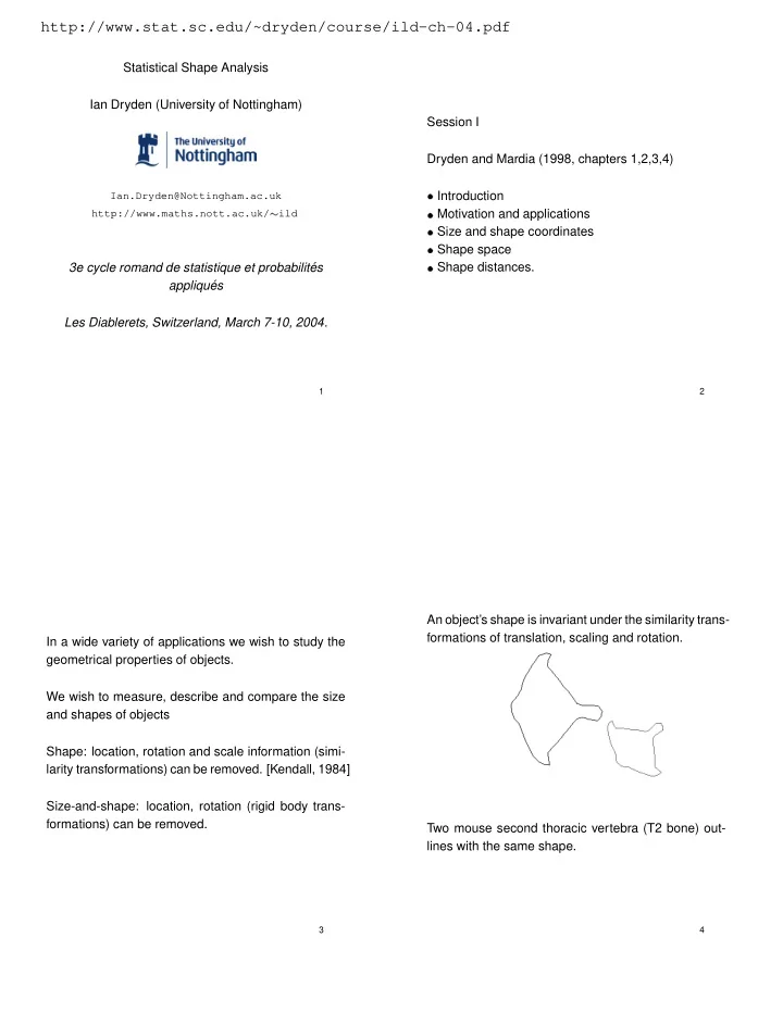
Pairwise plots: Size, shape distance, PC scores in direction of mean difference

s

0.03 0.05 0.07 f f f f f f f f f f f f f f f f f f f f f f f f f f f f f f m m m m m m m m m m m m m m m m m m m m m m mm m m m m m f

✩f ✩

f f f f f f f f ff f f f f f

✩

f f f f f f

✩ f f

f f f f f m m m m m m m m m m m m m m m m mm m m m m m m m m m m m

2 -1 0 1 2

f f f f f f f f f f f

✩

f

✩ f

f f

✩

f f

✩

f ff f f f f f f f ff f

✩

m m m m m m m m m m m m m m m m m m m m m m m m m m m mm f f f f f f f

✩

f f

✩

f f f f

✩

f f f f f

✩f f

f f f f f f f f f f m m m m m m m m m m m m m m m m m m m m m m m m m m m m m

3 -2 -1 0 1 2

f f

✩

f f f f f f

✩

f f f f f f f f f

✩

f f f f f ff f f f f f f m m m m m m m m m m m m m m m m m m m m m m m m m m mm m 240260280300 f f ff f ff f f f ff f f f f f f f f f f

✩

f f

✩

f f f

✩

f f f m m m m m m m m m m m m m m m m m m m m m m m m m m m m m 0.03 0.05

✪

0.07 f f f f f f f f f f f f f f f f f f f f f ff f f f f f f f m m m m m m m m m m m m m m m m m m m m m m m m m m m m m

dist

f

✩

f

✩

f f f f f f f f ff f f f f f

✩

f f f f f f

✩ f

f f f f f f m m m m m m m m m m m m m m m m m m m m m m m m m m m m m f f f f f f f f f f f

✩

f

✩ f

f f

✩

f f

✩

f f f f f f f f f f f f f

✩

m m m m m m m m m m m m m m m m m m m m m m m m m m m m m f f f f f f f

✩

f f

✩

f f f f

✩

f f f f f

✩f

f f f f f f f f f f f m m m m m m m m m m m m m m m m m m m m m m m m m m m m m f f

✩

f f f f f f

✩

f f f f f f f f f

✩

f f f f f ff f f f f f f m m m m m m m m m m m m m m m m m m m m m m m m m m m m m f f f f f f f f f f ff f f f ff f f f f f

✩

f f

✩

f f f

✩

f f f m m m m m m m m m m m m m m m m m m m m m mm m m m m m m ff f f f ff f f f f f f f f f f f f f f f f f f f f f f f m m m m m m m m m m m m m m m m m m m m m m m m m m m m m f f f f f f f f f f f f f f f ff f f f f f f f f f f f f f m m m m m m m m m m m m m m mm m m m m m m mm m m m m m

score 9

f f f f ff f f f f f

✩

f

✩

f f f

✩

f f

✩

f f f f f f f f f f f f f

✩

m m m m m m m m m m m m m m m m m m m m m m m m m m m m m f f f f f f f

✩

f f

✩

f f f f

✩

f f f f f

✩

f f f f f f f f f f f f m m m m mm m m m m m m m m m m m m m m m m m m m m m m m f f

✩

f f f f f f

✩

f f f f f f f f f

✩

f f f f f ff f f f f f f m m m m m m m m m m m m m m m m m m m m m m m m m m m m m

2

2 4 f f ff f ff f f f ff f f f ff f f f f f

✩

f f

✩

f f f

✩

f f f m m m m mm m m m m m m m m m m m m m m m mm m m m m m m

2 -1 0

✪

1 2

✫

ff f f f f f f f f f f f f f f f f f f f ff f f f f f ff m m m m m m m m m m m m m m m m m m mm m m m m m m m m m f f f f f f f f f f f f f f f f f f f f f f f f f f f f f f m m m m m m m m m m m m m m m m m m m m m m m m m m m m m f

✩

f

✩

f f f f f f f f f f f f f f f

✩

f f f f f f

✩

f f f f f f f m m m m m m mm m m m m m m m m m m m m m m m m m m m m m

score 11

f f f f f f f

✩

f f

✩

f f f f

✩

f f f f f

✩

f f f f f f f f f f f f m m m m mm m m m m m m m m m m m m m m m m m m m m m m m f f

✩

f f f f f f

✩

f f f f f f f f f

✩

f f f f f f f f f f f f f m m m m m m m m m m m m m m m m m m m m m m m m m m m m m f f ff f f f f f f f f f f f f f f f f f f

✩

f f

✩

f f f

✩

f f f m m m m mm m m m m m m m m m m m m m m m m m m m m m m m f f f f f ff f f f f f f f f f f f f f f f f f f f f f ff m m m m m m m m m m m m m m m m m m mm m m m m m m m m m f f f f f f f f f f f f f f f ff f f f f f f f f f f f f f m m m m m m m m m m m m m m mm m m m m m m mm m m m m m f

✩f ✩ f

f f f f f f f f f f f f f f

✩

f f f f f f

✩

f f f f f f f m m m m m m m m m m m m m m m m m m m m m m m m m m m m m f f f f ff f f f f f

✩

f

✩

f f f

✩

f f

✩

f ff f f f f f f f ff f

✩

m m m m m m m m m m m m m m m m m m m m m m m m m m m m m

score 2

f f

✩

f f f f f f

✩

f f f f f f f f f

✩

f f ff f f f f f f f f f m m m m m m m m m m m m m m m m m m m m m m m m m m m m m

2 -1 0 1 2 3

f f f f f ff f f f f f f f f ff f f f f f

✩

f f

✩

f f f

✩

f f f m m m m mm m m m m m m m m m m m m m m m mm m m m m m m

3 -2 -1 0 1 2

f f f f f ff f f f f f f f f f f f f f f f f f f f f f ff m m m m m m m m m m m m m m m m m m m m m m m m m m m m m f f f f f f f f f f f f f f f f f f f f f f f f f f f f f f m m m m m m m m m m m m m m m m m mm m m m mm m m m m m f

✩

f

✩

f f f f f f f f ff f f f f f

✩

f f f f f f

✩ f

f f f f f f m m m m m m mm m m m m m m m m mm m m m m m m m m m m m f f f f f f f f f f f

✩

f

✩ f

f f

✩

f f

✩

f ff f f f f f f f ff f

✩

m m m m m m m m m m m m m m m m m m m m m m m m m m m m m f f f f f f f

✩

f f

✩

f f f f

✩

f f f f f

✩

f f f f f f f f f f f f m m m m m m m m m m m m m m m m m m m m m m m m m m m m m

score 12

f f f f f ff f f f ff f f f f f f f f f f

✩

f f

✩

f f f

✩

f f f m m m m m m m m m m m m m m m m m m m m m mm m m m m m m 240260280300 f f f f f ff f f f f f f f f f f f f f f f f f f f f f f f m m m m m m m m m m m m m m m m m m m m m m m m m m m m m f f f f f f f f f f f f f f f ff f f f f f f f f f f f f f m m m m m m m m m m m m m m m m m mm m m m mm m m m m m

2

2

✬

4 f

✩

f

✩ f f

f f f f f f ff f f f f f

✩

f f f f f f

✩

f f f f f f f m m m m m m mm m m m m m m m m m m m m m m m m m m m m m f f f f ff f f f f f

✩

f

✩ f

f f

✩

f f

✩

f f f f f f f f f f f f f

✩

m m m m m m m m m m m m m m m m m m m m m m m m m m m m m

2 -1 0 1 2 3

f f f f f f f

✩

f f

✩

f f f f

✩

f f f f f

✩f

f f f f f f f f f f f m m m m mm m m m m m m m m m m m m m m m m m m m m m m m f f

✩

f f f f f f

✩

f f f f f f f f f

✩

f f f f f f f f f f f f f m mm m m m m m m m m m m m m m m m m m m m m m m m m m m

3 -2 -1 0 1 2

✬

3 -2 -1 0

✪

1 2

score 1

107

Goodall’s F test: If

➄ ✭ ✰ then ✥ ✟ Õ ❁ ✗ Õ ❂ ❀ ✮ Õ ❁ ✮ ❁ ✗ Õ ❂ ✮ ❁ ➷ ✮ ➬ ✚ ➹ Ø ✪ ✸ ➹ Ø ✮ ✛ ✯ Õ ❁ ★ ✩ ✪ ➷ ✮ ➬ ✚ ✆ ★ ✸ ➹ Ø ✪ ✛ ♦ ✯ Õ ❂ ★ ✩ ✪ ➷ ✮ ➬ ✚ ✯ ★ ✸ ➹ Ø ✮ ✛

Under

❧ ❙ : ✥ ✢ ✥ ï ◆ ❋ Õ ❁ ✗ Õ ❂ ❀ ✮ ■ ï ✁ Schizophrenia data: ✄ ✟ ✱ ❆

landmarks in

☎ ✟ t

dimensions

Ô ✪ ✟ ✱ ❺ ✸ Ô ✮ ✟ ✱ ❺ ✞ ✟ t ✄ ✬ ❺ ✟ t t ✥ ✟ ✱ ✶ Ñ ✦ , and ➅ ✚ ✥ ✮ ✮ ◆ ✰ ✱ ✮ ➆ ✱ ✶ Ñ ✦ ✛ í ❃ ✶ ❃ ✱

Permutation test: p-value = 0.04

✁ Hotelling’s ❻ ✮ test

p-value = 0.66

108

Comparing several groups: ANOVA Balanced analysis of variance with independent ran- dom samples

✚ ✆ ✫ ✪ ✸ ✶ ✶ ✶ ✸ ✆ ✫ Õ ✛ ✲ ✸ ❅ ✟ ✱ ✸ ✶ ✶ ✶ ✸ Ô ✲

from

Ô ✲

groups, each of size

Ô .

Let

➹ Ø ✫ be the group full Procrustes means and ➹ Ø

is the

verall pooled full Procrustes mean shape. A suitable

test statistic is

✥ ✟ Ô ✚ Ô ✬ ✱ ✛ Ô ✲ ✯ Õ ✳ ★ ✩ ✪ ➷ ✮ ➬ ✚ ➹ Ø ★ ✸ ➹ Ø ✛ ✚ Ô ✲ ✬ ✱ ✛ ✯ Õ ✳ ✫ ✩ ✪ ✯ Õ ★ ✩ ✪ ➷ ✮ ➬ ✚ ✆ ✫ ★ ✸ ➹ Ø ✫ ✛ ✶

Under

❧ ❙ ➃ equal mean shapes: ✥ ✢ ✥ ❋ Õ ✳ ❀ ✪ ■ ï ◆ Õ ✳ ❋ Õ ❀ ✪ ■ ï

and reject

❧ ❙ for large values of the statistic.

109

SLIDE 29

Complex Watson inference: Two independent random samples

❥ ✪ ✸ ✶ ✶ ✶ ✸ ❥ Õ from ✺ ❽ ✚ Ø ✸ ✌ ✛

and

✉ ✪ ✸ ✶ ✶ ✶ ✸ ✉ ☞

from

✺ ❽ ✚ ✴ ✸ ✌ ✛ . We wish to test be-

tween

❧ ❙ ➃ ➁ Ø ➂ ✟ ➁ ✴ ➂ ✴ ✑ ✒ ❧ ✪ ➃ ➁ Ø ➂ Ó ✟ ➁ ✴ ➂ ✸

where

➁ Ø ➂ ✟ ✖ ☞ ★ ✵ Ø ➃ ❃ ② ✶ ④ t ③ ✜ , (i.e. ➁ Ø ➂ rep-

resents the shape corresponding to the modal pre- shape

Ø . For large ✌

it follows that

Õ ✧ ★ ✩ ✪ ✔ ✏ ✑ ✮ ➵ ✚ ❥ ★ ✸ Ø ✛ ♦ ☞ ✧ ✫ ✩ ✪ ✔ ✏ ✑ ✮ ➵ ✚ ✉ ✫ ✸ ✴ ✛ í ✱ t ✌ ✜ ✮ ❋ ✮ ☛ ❀ ✈ ■ ❋ Õ ✗ ☞ ■

and we also have

Õ ✧ ★ ✩ ✪ ✔ ✏ ✑ ✮ ➵ ✚ ❥ ★ ✸ ➹ Ø ✛ ♦ ☞ ✧ ✫ ✩ ✪ ✔ ✏ ✑ ✮ ➵ ✚ ✉ ✫ ✸ ➹ ✴ ✛ í ✱ t ✌ ✜ ✮ ❋ ✮ ☛ ❀ ✈ ■ ❋ Õ ✗ ☞ ❀ ✮ ■

110

By analogy with analysis of variance we can write

Õ ✧ ★ ✩ ✪ ✔ ✏ ✑ ✮ ➵ ✚ ❥ ★ ✸ ➹ ➹ Ø ✛ ♦ ☞ ✧ ✫ ✩ ✪ ✔ ✏ ✑ ✮ ➵ ✚ ✉ ✫ ✸ ➹ ➹ Ø ✛ ✟ Õ ✧ ★ ✩ ✪ ✔ ✏ ✑ ✮ ➵ ✚ ❥ ★ ✸ ➹ Ø ✛ ♦ ☞ ✧ ✫ ✩ ✪ ✔ ✏ ✑ ✮ ➵ ✚ ✉ ✫ ✸ ➹ ✴ ✛ ♦ æ

where

➹ ➹ Ø

is the overall MLE of

Ø

if the two groups are pooled, and

æ

is analogous to the between sum of

squares. Since,

Õ ✧ ★ ✩ ✪ ✔ ✏ ✑ ✮ ➵ ✚ ❥ ★ ✸ ➹ ➹ Ø ✛ ♦ ☞ ✧ ✫ ✩ ✪ ✔ ✏ ✑ ✮ ➵ ✚ ✉ ✫ ✸ ➹ ➹ Ø ✛ í ✱ t ✌ ✜ ✮ ❋ ✮ ☛ ❀ ✈ ■ ❋ Õ ✗ ☞ ❀ ✪ ■

it follows that

æ ✟ Õ ✧ ★ ✩ ✪ ✔ ✏ ✑ ✮ ➵ ✚ ❥ ★ ✸ ➹ ➹ Ø ✛ ♦ ☞ ✧ ✫ ✩ ✪ ✔ ✏ ✑ ✮ ➵ ✚ ✉ ✫ ✸ ➹ ➹ Ø ✛ ✬ Õ ✧ ★ ✩ ✪ ✔ ✏ ✑ ✮ ➵ ✚ ❥ ★ ✸ ➹ Ø ✛ ✬ ☞ ✧ ✫ ✩ ✪ ✔ ✏ ✑ ✮ ➵ ✚ ✉ ✫ ✸ ➹ ✴ ✛ í ✱ t ✌ ✜ ✮ ✮ ☛ ❀ ✈ ✶

111

Therefore, under

❧ ❙ we have ✥ ✮ ✟ ✚ Ô ♦ ☎ ✬ t ✛ æ ✯ Õ ★ ✩ ✪ ✔ ✏ ✑ ✮ ➵ ✚ ❥ ★ ✸ ➹ Ø ✛ ♦ ✯ ☞ ✫ ✩ ✪ ✔ ✏ ✑ ✮ ➵ ✚ ✉ ✫ ✸ ➹ ✴ ✛ í ✥ ✮ ☛ ❀ ✈ ◆ ❋ ✮ ☛ ❀ ✈ ■ ❋ Õ ✗ ☞ ❀ ✮ ■

and so we reject

❧ ❙

for large values of

✥ ✮ . Using

Taylor series expansions for large concentrations

æ í ✚ Ô ❀ ✪ ♦ ☎ ❀ ✪ ✛ ❀ ✪ ✔ ✏ ✑ ✮ ➵ ✚ ➹ Ø ✸ ➹ ✴ ✛ ✸

and so for large

✌

the test statistic

✥ ✮ is equivalent to

the two sample test statistic of Goodall (1991). Bayesian approach to inference

③ ✚ ✷ ✸ ➄ ➸ ✼ ✪ ✸ ✶ ✶ ✶ ✸ ✼ Õ ✛ ✟ ✸ ✚ ✼ ✪ ✸ ✶ ✶ ✶ ✸ ✼ Õ ⑨ ✷ ✸ ➄ ✛ ③ ✚ ✷ ✸ ➄ ✛ ✹ ✸ ✚ ✼ ✪ ✸ ✶ ✶ ✶ ✸ ✼ Õ ⑨ ✷ ✸ ➄ ✛ ③ ✚ ✷ ✸ ➄ ✛ ✒ ✷ ✒ ➄ ✶

e.g. Data

❥ ★ ✢

complex Watson(

Ø , ✌

known ) Prior

Ø ✢

complex Bingham (

⑩

known)

③ ✚ Ø ➸ ❥ ✪ ✸ ✶ ✶ ✶ ✸ ❥ Õ ✛ ✭ ③ ✚ Ø ✛ ✸ ✚ ❥ ✪ ✸ ✶ ✶ ✶ ✸ ❥ Õ ✛ ✭ ✓ ☛ Û ✺ ✻ ✼ Ø ➼ ⑩ Ø ♦ ✌ Õ ✧ ★ ✩ ✪ ❥ ➼ ★ Ø Ø ➼ ❥ ★ ✽ ✾ ✿ ✟ ✓ ☛ Û ✖ Ø ➼ ✚ ✌ ✘ ♦ ⑩ ✛ Ø ✜ ✸

Conjugate prior MAP: dominant eigenvector of

✘ ♦ ⑩ r ✌

112

SLIDE 30

The smoothed Procrustes mean of the T2 Small data: (Top left)

➩ ✟ ❃ , (top right) ➩ ✟ ❃ ✶ ✱ , (bottom left) ➩ ✟ ✱ ✶ ❃ , (bottom right) ➩ ✟ ✱ ❃ ❃ .

113

EDMA (Euclidean distance matrix analysis) [Lele, 91+, Stoyan, 91]

✥ ✚ ✆ ✛ : form distance matrix ( ✄ ✝ ✄ matrix of pairs of

inter-landmark distances (ILDs)) Estimate

✥ ✚ Ø ✛ : population form distance matrix ✚ ✷ ✫ ✸ ✉ ✫ ✛ ✢ ✣ ✚ ✚ Ø ✫ ✸ ✴ ✫ ✛ ✸ ✍ ✮ ✰ ✮ ✛ ✸ ❅ ✟ ✱ ✸ ✶ ✶ ✶ ✸ ✄ . Then ✚ ✷ ❀ ✬ ✷ ❁ ✛ ✮ ♦ ✚ ✉ ❀ ✬ ✉ ❁ ✛ ✮ ✟ ✵ ✮ ❀ ❁ ✢ ✍ ✮ ✜ ✮ ✮ ✚ ❂ ✮ ❀ ❁ r ✍ ✮ ✛ ✸ (4) ❂ ✮ ❀ ❁ ✟ ✚ Ø ❀ ✬ Ø ❁ ✛ ✮ ♦ ✚ ✴ ❀ ✬ ✴ ❁ ✛ ✮ .

Moment estimator

❂ ✈ ❀ ❁ ✟ ✖ ✠ ✚ ✵ ✮ ❀ ❁ ✛ ✜ ✮ ✬ ❃ ✴ ✳ ✚ ✵ ✮ ❀ ❁ ✛ ✶

Removes bias. Estimate of mean reflection size-and-shape

➁ ✞ ✵ ✘ ✮ ✚ ❄ ✛ ➂ ✸ ✚ ❄ ✛ ❀ ❁ ✟ ➹ ❂ ❀ ❁ ✸

114

EDMA-I test (Lele and Richtsmeier, 1991) Form ratio distance matrix

✵ ★ ✫ ✚ ✆ ✸ ✯ ✛ ✟ ✥ ★ ✫ ✚ ✆ ✛ r ✥ ★ ✫ ✚ ✯ ✛ ✶

(5) Test statistic:

❻ ✟ ❅ ✴ ☛ ★ ◆ ✫ ✵ ★ ✫ ✚ ➹ Ø ✸ ➹ ✴ ✛ r ❅ ✏ ✑ ★ ◆ ✫ ✵ ★ ✫ ✚ ➹ Ø ✸ ➹ ✴ ✛ ✸

(6) Use bootstrap procedures.

115

EDMA-II (Lele and Cole, 1995)

➹ ✥ Ù

and

➹ ✥ ❆ estimates of average form distance matrix

for each group Scale by group size measure

❻

= Largest entry in arithmetic difference of scaled matrices More powerful than EDMA-I

116

SLIDE 31

Rao and Suryawanshi (1996)

❇ ✚ ✆ ✛ : form log-distance matrix

shape log-distance matrix is

❇ ➼ ✚ ✆ ✛ ✟ ❇ ✚ ✆ ✛ ✬ ✭ ❇ ✱ ☛ ✱ ➻ ☛ ✸ ✭ ❇ ✟ t ✄ ✚ ✄ ✬ ✱ ✛ ☛ ❀ ✪ ✧ ★ ✩ ✪ ☛ ✧ ✫ ✩ ★ ✗ ✪ ✚ ❇ ✚ ✆ ✛ ✛ ★ ✫ ✶

Average form log-distance matrix is

❇ ✚ ➹ Ø ✛ ✟ ✱ Ô Õ ✧ ★ ✩ ✪ ❈ ✎ ➴ ➷ ★ ✚ ❾ ✪ ✸ ❾ ✮ ✛ ✸

where

➷ ★ ✚ ❾ ✪ ✸ ❾ ✮ ✛ is the distance between landmarks ❾ ✪ and ❾ ✮ for the ♣ th object ✆ ★ .

Average reflection size-and-shape

➁ ✞ ✵ ✘ ☞ ✚ ✓ ☛ Û ✚ ❇ ✚ ➹ Ø ✛ ✛ ✛ ➂ ✶

117

Average reflection shape

➁ ✞ ✵ ✘ ☞ ✚ ✓ ☛ Û ✚ ❇ ➼ ✚ ➹ Ø ✛ ✛ ✛ ➂ ✶

For small variations estimates of mean shape or size- and-shape are all very similar...(Kent, 1994) Distance based (+): Landmarks not necessarily needed (eg. maximum breadth) Consistent estimation under general normal models Distance based (-): Invariant under reflections Visualization not straightforward A choice of metric for averaging needs to be made

118

✁ SIZE-AND-SHAPE

Invariance under translation and rotation (not scale) Perturbation model:

✆ ★ ✟ ✚ Ø ♦ ✠ ★ ✛ ❼ ★ ♦ ✱ ☛ Ö ➻ ★ ✸ ♣ ✟ ✱ ✸ ✶ ✶ ✶ ✸ Ô ✸ ✁ ALLOMETRY

The relationship of shape given size

119

SLIDE 32

Bookstein’s (1996) Microfossils

U

V

❱

0.2 0.3 0.4 0.5 0.6 0.4 0.5 0.6 0.7 0.8 60 65 64 65 67 71 72 71 74 75 76 84 84 84 87 88 88 88 92 100 100

✐ ✟ ✐ ✽

versus

❤ ✟ ❤ ✽ ♦ ✱ r t

120

Microfossils:

slog

0.32 0.36 0.40 0.44

•
•
8.2

8.4 8.6 8.8 9.0

❳

9.2

•
0.32

0.36 0.40 0.44

•
U
•
8.2

8.4 8.6 8.8 9.0 9.2

❉

•
0.45

0.55 0.65 0.75 0.45 0.55

❨

0.65 0.75

V

Regression:

❤ ✟ ✶ ✪ ♦ ➾ ✪ ❈ ✎ ➴ ✘ ✸ ✐ ✟ ✶ ✮ ♦ ➾ ✮ ❈ ✎ ➴ ✘

Tthe fitted values (with standard errors) are

➹ ✶ ✪ ✟ ❃ ✶ Ò Ò ✚ ❃ ✶ t ❃ ✛ , ➹ ➾ ✪ ✟ ✬ ❃ ✶ ❃ ❺ ✚ ❃ ✶ ❃ t ✛ , ➹ ✶ ✮ ✟ ✬ ✱ ✶ ❺ Ò ✚ ❃ ✶ ❆ t ✛ and ➹ ➾ ✮ ✟ ❃ ✶ t ❺ ✚ ❃ ✶ ❃ ❺ ✛

Significant linear relationship between

❈ ✎ ➴ ✘

and

✐

.

121

T2 Small mouse vertebrae data

s

0.10
0.05

0.0 0.05

0.02

0.0 0.02 165 170 175 180 185

0.10
0.05

0.0 0.05

PC1
•
PC2
0.04 -0.02

0.0 0.02

165 170 175 180 185
0.02

0.0 0.02

0.04 -0.02

0.0 0.02

PC3

NB: Approx. linear relationship between PC 1 and centroid size.

122

Shapes package in R: http://www.cran-r-project.org Library of shape analysis routines. Also see: http://www.maths.nott.ac.uk/

✢ ild/shapes

123

SLIDE 33

Session III:

✁ Deformations ✁ Shape in images ✁ Temporal shape ✁ Shape Regression ✁ Discussion

124

DEFORMATIONS AND THIN-PLATE SPLINES The thin-plate spline is the most natural interpolant in two dimensions because it minimizes the amount of bending in transforming between two configurations, which can also be considered a roughness penalty. The theory of which was developed by Duchon (1976) and Meinguet (1979). Consider the

✚ t ✝ ✱ ✛ landmarks ✓ ✫ ✸ ❅ ✟ ✱ ✸ ✶ ✶ ✶ ✸ ✄ , on the first figure mapped exactly

into

✉ ★ ✸ ♣ ✟ ✱ ✸ ✶ ✶ ✶ ✸ ✄ , on the second figure, i.e. there

are

t ✄

interpolation constraints,

✚ ✉ ✫ ✛ ❀ ✟ ❊ ❀ ✚ ✓ ✫ ✛ ✸ s ✟ ✱ ✸ t ✸ ❅ ✟ ✱ ✸ ✶ ✶ ✶ ✸ ✄ ✸

(7) and we write

❊ ✚ ✓ ✫ ✛ ✟ ✚ ❊ ✪ ✚ ✓ ✫ ✛ ✸ ❊ ✮ ✚ ✓ ✫ ✛ ✛ ➻ ✸ ❅ ✟ ✱ ✸ ✶ ✶ ✶ ✸ ✄ ✸

for the two dimensional deformation. Let

❻ ✟ ➁ ✓ ✪ ✓ ✮ ✶ ✶ ✶ ✓ ☛ ➂ ➻ ✸ ✯ ✟ ➁ ✉ ✪ ✉ ✮ ✶ ✶ ✶ ✉ ☛ ➂ ➻

so that

❻

and

✯

are both

✚ ✄ ✝ t ✛ matrices.

A pair of thin-plate splines (PTPS) is given by the bivariate function

❊ ✚ ✓ ✛ ✟ ✚ ❊ ✪ ✚ ✓ ✛ ✸ ❊ ✮ ✚ ✓ ✛ ✛ ➻ ✟ ô ♦ ⑩ ✓ ♦ ❽ ➻ ò ✚ ✓ ✛ ✸

(8)

125

where

✓ is ✚ t ✝ ✱ ✛ ✸ ò ✚ ✓ ✛ ✟ ✚ ✍ ✚ ✓ ✬ ✓ ✪ ✛ ✸ ✶ ✶ ✶ ✸ ✍ ✚ ✓ ✬ ✓ ☛ ✛ ✛ ➻ ✸ ✚ ✄ ✝ ✱ ✛ and ✍ ✚ ❾ ✛ ✟ ❮ ✤ ❾ ✤ ✮ ❈ ✎ ➴ ✚ ✤ ❾ ✤ ✛ ✸ ✤ ❾ ✤ ➆ ❃ ✸ ❃ ✸ ✤ ❾ ✤ ✟ ❃ ✶

(9) The

t ✄ ♦ ✧

parameters of the mapping are

ô ✚ t ✝ ✱ ✛ ✸ ⑩ ✚ t ✝ t ✛ and ❽ ✚ ✄ ✝ t ✛ . There are t ✄

interpola- tion constraints in Equation (7), and we introduce six more constraints in order for the bending energy in Equation (14) below to be defined:

✱ ➻ ☛ ❽ ✟ ❃ ✸ ❻ ➻ ❽ ✟ ❃ ✶

(10) The pair of thin-plate splines which satisfy the con- straints of Equation (10) are called natural thin-plate

splines. Equations (7) and (10) can be re-written in

matrix form

❋

❍

✘ ✱ ☛ ❻ ✱ ➻ ☛ ❃ ❃ ❻ ➻ ❃ ❃ ■ ❏ ❑ ❋

❍

❽ ô ➻ ⑩ ➻ ■ ❏ ❑ ✟ ❋

❍

✯ ❃ ❃ ■ ❏ ❑ ✸

(11) where

✚ ✘ ✛ ★ ✫ ✟ ✍ ✚ ✓ ★ ✬ ✓ ✫ ✛ and ✱ ☛

is the

✄ -vector of

nes. The matrix

❼ ✟ ❋

❍

✘ ✱ ☛ ❻ ✱ ➻ ☛ ❃ ❃ ❻ ➻ ❃ ❃ ■ ❏ ❑

is symmetric positive definite and so the inverse ex- ists, provided the inverse of

✘

exists. Hence,

❋

❍

❽ ô ➻ ⑩ ➻ ■ ❏ ❑ ✟ ❋

❍

✘ ✱ ☛ ❻ ✱ ➻ ☛ ❃ ❃ ❻ ➻ ❃ ❃ ■ ❏ ❑ ❀ ✪ ❋

❍

✯ ❃ ❃ ■ ❏ ❑ ✟ ❼ ❀ ✪ ❋

❍

✯ ❃ ❃ ■ ❏ ❑ ✸

say. Writing the partition of

❼ ❀ ✪

as

❼ ❀ ✪ ✟ ▲ ❼ ✪ ✪ ❼ ✪ ✮ ❼ ✮ ✪ ❼ ✮ ✮ ▼ ✸

where

❼ ✪ ✪

is

✄ ✝ ✄ , it follows that ❽ ✟ ❼ ✪ ✪ ✯ ▲ ô ➻ ⑩ ➻ ▼ ✟ ➁ ➹ ➾ ✪ ✸ ➹ ➾ ✮ ➂ ✟ ❼ ✮ ✪ ✯ ✸

(12) giving the parameter values for the mapping. If

✘ ❀ ✪

SLIDE 34

exists, then we have

❼ ✪ ✪ ✟ ✘ ❀ ✪ ✬ ✘ ❀ ✪ ◆ ✚ ◆ ➻ ✘ ❀ ✪ ◆ ✛ ❀ ✪ ◆ ➻ ✘ ❀ ✪ ✸ ❼ ✮ ✪ ✟ ✚ ◆ ➻ ✘ ❀ ✪ ◆ ✛ ❀ ✪ ◆ ➻ ✘ ❀ ✪ ✟ ✚ ❼ ✪ ✮ ✛ ➻ ✸

(13)

❼ ✮ ✮ ✟ ✬ ✚ ◆ ➻ ✘ ❀ ✪ ◆ ✛ ❀ ✪ ✸

where

◆ ✟ ➁ ✱ ☛ ✸ ❻ ➂ , using for example Rao (1973,p39).

Using Equations (12) and (13) we see that

➹ ➾ ✪ and ➹ ➾ ✮

are generalized least squares estimators, and

✍ ✎ ❃ ✚ ✚ ➹ ➾ ✪ ✸ ➹ ➾ ✮ ✛ ➻ ✛ ✟ ✬ ❼ ✮ ✮ ✶

Mardia et al. (1991) gave the expressions for the case when

✘

is singular. The

✄ ✝ ✄

matrix

æ ❖

is called the bending energy matrix where

æ ❖ ✟ ❼ ✪ ✪ ✶

(14) There are three constraints on the bending energy matrix

✱ ➻ ☛ æ ❖ ✟ ❃ ✸ ❻ ➻ æ ❖ ✟ ❃

and so the rank of the bending energy matrix is

✄ ✬ ❆ .

It can be proved that the transformation of Equation (8) minimizes the total bending energy of all possible interpolating functions mapping from

❻

to

✯

, where the total bending energy is given by

P ✚ ❊ ✛ ✟ ✮ ✧ ✫ ✩ ✪ ◗ ◗ ❘ ❙ ❂ ❶ ❚ ✮ ❊ ✫ ❚ ✷ ✮ ❷ ✮ ♦ t ❶ ❚ ✮ ❊ ✫ ❚ ✷ ❚ ✉ ❷ ✮ ♦ ❶ ❚ ✮ ❊ ✫ ❚ ✉ ✮ ❷ ✮ ✒ ✷ ✒ ✉ ✶

(15) A simple proof is given by Kent and Mardia (1994a). The minimized total bending energy is given by,

P ✚ ❊ ✛ ✟ ✕ ✳ ✴ ✍ ✓ ✚ ❽ ➻ ✘ ❽ ✛ ✟ ✕ ✳ ✴ ✍ ✓ ✚ ✯ ➻ ❼ ✪ ✪ ✯ ✛ ✶

(16) In calculating a deformation grid we do not want to see any more bending locally than is necessary and also do not want to see bending where there are no data. Early transformation grids of human profiles

126

Early transformation grids modelling six stages through life (from Medawar, 1944).

127

SLIDE 35

TRANSFORMA TION GRIDS Following from the original ideas of D’Arcy Thompson (1917) we can produce similar transformation grids, using a pair of thin-plate splines for the deformation from configuration matrices

❻

to

✯

.

(a) (b)

128

A regular square grid is drawn over the first figure and at each point where two lines on the grid meet

✓ ★ the

corresponding position in the second figure is calcu- lated using a pair of thin-plate splines transformation

✉ ★ ✟ ❊ ✚ ✓ ★ ✛ ✸ ♣ ✟ ✱ ✸ ✶ ✶ ✶ ✸ Ô ❯ , where Ô ❯

is the number

f junctions or crossing points on the grid. The junc-

tion points are joined with lines in the same order as in the first figure, to give a deformed grid over the sec-

nd figure. The pair of thin-plate splines can be used

to produce a transformation grid, say from a regular square grid on the first figure to a deformed grid on the second figure. The resulting interpolant produces transformation grids that ‘bend’ as little as possible. We can think of each square in the deformation as be- ing deformed into a quadrilateral (with four shape pa- rameters). The PTPS minimizes the local variation of these small quadrilaterals with respect to their neigh- bours. Consider describing the square to kite transformation which was considered by Bookstein (1989) and Mardia and Goodall (1993). Given

✄ ✟ ❺ points in ☎ ✟ t dimensions the ma-

trices

❻

and

✯

are given by

❻ ✟ ❋

❍

❃ ✱ ✬ ✱ ❃ ❃ ✬ ✱ ✱ ❃ ■ ❏ ❏ ❏ ❑ ✸ ✯ ✟ ❋

❍

❃ ❃ ✶ Ò ❄ ✬ ✱ ❃ ✶ t ❄ ❃ ✬ ✱ ✶ t ❄ ✱ ❃ ✶ t ❄ ■ ❏ ❏ ❏ ❑ ✶

We have here

✘ ✟ ❋

❍

❃ ✣ ➽ ✣ ✣ ❃ ✣ ➽ ➽ ✣ ❃ ✣ ✣ ➽ ✣ ❃ ■ ❏ ❏ ❏ ❏ ❑ ✸

where

✣ ✟ ✍ ✚ ✦ t ✛ ✟ ❃ ✶ ✧ ✦ ❆ ✱

and

➽ ✟ ✍ ✚ t ✛ ✟ t ✶ Ò Ò t ✧ . In this case, the bending energy matrix is æ ❖ ✟ ❼ ✪ ✪ ✟ ❃ ✶ ✱ Ñ ❃ ❆ ❋

❍

✱ ✬ ✱ ✱ ✬ ✱ ✬ ✱ ✱ ✬ ✱ ✱ ✱ ✬ ✱ ✱ ✬ ✱ ✬ ✱ ✱ ✬ ✱ ✱ ■ ❏ ❏ ❏ ❑ ✶

129

It is found that

❽ ➻ ✟ ▲ ❃ ❃ ❃ ❃ ✬ ❃ ✶ ✱ Ñ ❃ ❆ ❃ ✶ ✱ Ñ ❃ ❆ ✬ ❃ ✶ ✱ Ñ ❃ ❆ ❃ ✶ ✱ Ñ ❃ ❆ ▼ ✸(17) ô ✟ ❃ ✸ ⑩ ✟ ✰ ✮

and so the pair of thin-plate splines is given by

❊ ✚ ✓ ✛ ✟ ✚ ❊ ✪ ✚ ✓ ✛ ✸ ❊ ✮ ✚ ✓ ✛ ✛ ➻ , where ❊ ✪ ✚ ✓ ✛ ✟ ✓ ➁ ✱ ➂ ✸

(18)

❊ ✮ ✚ ✓ ✛ ✟ ✓ ➁ t ➂ ♦ ❃ ✶ ✱ Ñ ❃ ❆ ✈ ✧ ✫ ✩ ✪ ✚ ✬ ✱ ✛ ✫ ✍ ✚ ✤ ✓ ✬ ✓ ✫ ✤ ✛ ✶

Note that Equation (18) is as expected, because there is no change in the

✓ ➁ ✱ ➂ direction. The affine part of the defor-

mation is the identity transformation.

SLIDE 36

2
1

1 2

2
1

1 2

2
1

1 2

2
1

1 2

2
1

1 2

2
1

1 2

2
1

1 2

2
1

1 2

Transformation grids for the square (left column) to kite

(right column) (after Bookstein, 1989). In the second row the same figures as in the first row have been rotated by

❺ ❄ ♠

and the deformed grid does look different, even though the transformation is the same. We consider Thompson-like grids for this example (above). A regular square grid is placed on the first figure and de- formed into the curved grid on the kite figure. We see that the top and bottom most points are moved downwards with respect to the other two points. If the regular grid is drawn

n the first figure at a different orientation, then the de-

formed grid does appear to be different, even though the transformation is the same. This effect is seen in the Figure where both figures have been rotated clockwise by

❺ ❄ ♠ in

the second row.

0.6 -0.4 -0.2 0.0

(a) 0.2 0.4 0.6

0.6 -0.4 -0.2 0.0

0.2 0.4 0.6

•
0.6 -0.4 -0.2 0.0

(b) 0.2 0.4 0.6

0.6 -0.4 -0.2 0.0

0.2 0.4 0.6

•
A thin-plate spline transformation grid between the con-

trol mean shape estimate and the schizophrenia mean shape estimate. (left) We see a square grid drawn on the estimate of mean shape for the Control group in the schizophrenia

study. Here there are

Ô ❯ ✟ ❆ ❃ ✝ t ✦ ✟ Ñ Ò ❃

junctions and there are

✄ ✟ ✱ ❆

landmarks. (right) we see the

schizophrenia mean shape estimate and the grid of new points obtained from the PTPS transformation. It is quite clear that there is a shape change in the centre of the brain, around landmarks 1, 9 and 13.

130

6000 7000 8000 9000 10000 11000 12000 8000 9000 10000 11000 12000 13000

6000

7000 8000 9000 10000 11000 12000 8000 9000 10000 11000 12000 13000

6000

7000 8000 9000 10000 11000 12000 8000 9000 10000 11000 12000 13000

6000

7000 8000 9000 10000 11000 12000 8000 9000 10000 11000 12000 13000

6000

7000 8000 9000 10000 11000 12000 8000 9000 10000 11000 12000 13000

A series of grids showing the shape changes in the

skull of some sooty mangabey monkeys

131

SLIDE 37

PRINCIPAL AND PARTIAL WARPS Bookstein (1989, 1991)’s principal and partial warps are useful for decomposing the thin-plate spline trans- formations into a series of large scale and small scale components. Consider the pair of thin-plate splines transformation from

✓ ✹ ✠ ✡ ✮

to

✉ ✹ ✠ ✡ ✮ , which interpolates the ✄

points

❻

to

✯

(

✄ ✝ t ) matrices. An eigen-decomposition

f the

✄ ✝ ✄ bending energy matrix æ ❖ of Equation (14)

has non-zero eigenvalues

➩ ✪ ② ➩ ✮ ② ✶ ✶ ✶ ② ➩ ☛ ❀ P

with corresponding eigenvectors

Ö ✪ ✸ Ö ✮ ✸ ✶ ✶ ✶ ✸ Ö ☛ ❀ P . The

eigenvectors

Ö ✪ ✸ Ö ✮ ✸ ✶ ✶ ✶ ✸ Ö ☛ ❀ P

are called the princi- pal warp eigenvectors and the eigenvalues are called the bending energies. The functions,

➅ ✫ ✚ ✓ ✛ ✟ Ö ➻ ✫ ò ✚ ✓ ✛ ✸ ❅ ✟ ✱ ✸ ✶ ✶ ✶ ✸ ✄ ✬ ❆ ✸

are the principal warps, where

ò ✚ ✓ ✛ ✟ ✚ ✍ ✚ ✓ ✬ ✓ ✪ ✛ ✸ ✶ ✶ ✶ ✸ ✍ ✚ ✓ ✬ ✓ ☛ ✛ ✛ ➻ .

132

Here we have labelled the eigenvalues and eigenvec- tors in this order (with

➩ ✪ as the smallest eigenvalue

corresponding to the first principal warp) to follow Book- stein’s (1996b) labelling of the order of the warps. The principal warps do not depend on the second figure

✯

. The principal warps will be used to construct an or- thogonal basis for re-expressing the thin-plate spline

transformations. The principal warp deformations are

univariate functions of two dimensional

✓ , and so could

be displayed as surfaces above the plane or as con- tour maps. Alternatively one could plot the transfor- mation grids from

✓ to ✉ ✟ ✓ ♦ ✚ ô ✪ ➅ ✫ ✚ ✓ ✛ ✸ ô ✮ ➅ ✫ ✚ ✓ ✛ ✛ ➻

for each

❅ , for particular values of ô ✪ and ô ✮ . Note that

the principal warps are orthonormal. The partial warps are defined as the set of

✄ ✬ ❆

bivariate functions

é ✫ ✚ ✓ ✛ ✸ ❅ ✟ ✱ ✸ ✶ ✶ ✶ ✸ ✄ ✬ ❆ , where é ✫ ✚ ✓ ✛ ✟ ✯ ➻ ➩ ✫ Ö ✫ ➅ ✫ ✚ ✓ ✛ ✟ ✯ ➻ ➩ ✫ Ö ✫ Ö ➻ ✫ ò ✚ ✓ ✛ ✶

The

❅ th partial warp scores for ✯

(from

❻ ) are de-

fined as

✚ ó ✫ ✪ ✸ ó ✫ ✮ ✛ ➻ ✟ ✯ ➻ Ö ✫ ✸ ❅ ✟ ✱ ✸ ✶ ✶ ✶ ✸ ✄ ✬ ❆ ✸

and so there are two scores for each partial warp. Since

❽ ➻ ò ✚ ✓ ✛ ✟ ☛ ❀ P ✧ ✫ ✩ ✪ é ✫ ✚ ✓ ✛ ✸

we see that the non-affine part of the pair of thin-plate splines transformation can be decomposed into the sum of the partial warps. The

❅ th partial warp cor-

responds largely to the movement of the landmarks which are the most highly weighted in the

❅ th prin-

cipal warp. The

❅ th partial warp scores indicate the

contribution of the

❅ th principal warp to the deforma-

tion from the source

❻

to the target

✯

, in each of the Cartesian axes.

0.6
0.4
0.2

0.0 0.2 0.4 0.6

0.6
0.4
0.2

0.0 0.2 0.4 0.6

0.6
0.4
0.2

0.0 0.2 0.4 0.6

0.6
0.4
0.2

0.0 0.2 0.4 0.6

0.6
0.4
0.2

0.0 0.2

❱

0.4 0.6

0.6
0.4
0.2

0.0 0.2 0.4 0.6

0.6
0.4
0.2

0.0 0.2 0.4 0.6

0.6
0.4
0.2

0.0 0.2 0.4 0.6

0.6
0.4
0.2

0.0 0.2 0.4 0.6

0.6
0.4
0.2

0.0 0.2 0.4 0.6

•
The five principal warps for the the pooled mean shape
f the gorillas

133

SLIDE 38

0.6 -0.4 -0.2 0.0

(a) 0.2 0.4 0.6

0.6 -0.4 -0.2 0.0

0.2 0.4 0.6

0.6 -0.4 -0.2 0.0

(b) 0.2 0.4 0.6

0.6 -0.4 -0.2 0.0

0.2 0.4 0.6

A thin-plate spline transformation grid between a fe-

male and a male gorilla skull midline.

134

0.6
0.4
0.2

0.0 0.2 0.4 0.6

0.6
0.4
0.2

0.0 0.2 0.4

0.6
•
0.6
0.4
0.2

0.0 0.2

ö

0.4 0.6

0.6
0.4
0.2

0.0 0.2 0.4

0.6
0.6
0.4
0.2

0.0 0.2 0.4 0.6

0.6
0.4
0.2

0.0 0.2 0.4

0.6
0.6
0.4
0.2

0.0 0.2 0.4 0.6

0.6
0.4
0.2

0.0 0.2 0.4 0.6

•
0.6
0.4
0.2

0.0 0.2

ö

0.4 0.6

0.6
0.4
0.2

0.0 0.2 0.4 0.6

•
0.6
0.4
0.2

0.0 0.2 0.4 0.6

0.6
0.4
0.2

0.0 0.2 0.4 0.6

Affine and partial warps for Gorilla (Female to male

mean shapes)

135

f f f f f f f f f f f f f f f f f f f f f f f f f f f f f f

0.06 -0.04 -0.02

0.0 0.02 0.04 0.06

0.06
0.04 -0.02

0.0 0.02 0.04 0.06 m m m m m m m m m m m m m m m m m m m m m m m m m m m m m f ff f f f f f f f f f f f f f f f f f f f f f f f f f f f

0.06 -0.04 -0.02

0.0 0.02 0.04 0.06

0.06
0.04 -0.02

0.0 0.02 0.04 0.06 m m m m m m m m m m m m m m m m m m m m m m m m m m m m m f f f f f f f f f f f f f f f f f f f f f f f f f ff f f f

0.06 -0.04 -0.02

0.0 0.02 0.04 0.06

0.06
0.04 -0.02

0.0 0.02 0.04 0.06 m m m m m m m m m m m m m m m m m m m m m m m m m m m m m f f f f f f f f f f f f f f f f f f f f f f f f f f f f f f

0.06 -0.04 -0.02

0.0 0.02 0.04 0.06

0.06 -0.04 -0.02

0.0 0.02 0.04 0.06 m m m m m m m m m m m m m m m m m m m m m m m m m m m m m f f f f f f f f f f f f f f f f f f f f f f f f f f f f f f

0.06 -0.04 -0.02

0.0 0.02 0.04 0.06

0.06 -0.04 -0.02

0.0 0.02 0.04 0.06 m m m m mm m m m m m m m m m m m m m m m m m m m m m m m f f f f f f f f f f f f f fff f f f f f f f f ff f f f f

0.06 -0.04 -0.02

0.0 0.02 0.04 0.06

0.06 -0.04 -0.02

0.0 0.02 0.04 0.06 m m m m m m m m m m m m m m m m m m m m m m m m mm m m m

Affine scores and the partial warp scores for female (f) and male (m) gorilla skulls.

136

RELATIVE WARPS Principal component analysis with non-Euclidean met- rics Define the pseudo-metric space

✚ ✠ ✡ è ✸ ➷ ð ✛ as the real ó -vectors with pseudo-metric given by ➷ ð ✚ ✷ ✪ ✸ ✷ ✮ ✛ ✟ ❲ ✚ ✷ ✪ ✬ ✷ ✮ ✛ ➻ ⑩ ❀ ✚ ✷ ✪ ✬ ✷ ✮ ✛ ✸

where

✷ ✪

and

✷ ✮

are

ó -vectors, and ⑩ ❀

is a gener- alized inverse (or inverse if it exists) of the positive semi-definite matrix

⑩ .

The Moore–Penrose inverse is a suitable choice of generalized inverse. If

⑩

is the population covariance matrix of

✷ ✪

and

✷ ✮ , then ➷ ð ✚ ✷ ✪ ✸ ✷ ✮ ✛

is the Maha- lanobis distance. The norm of a vector

✷

in the metric space is

✤ ✷ ✤ ð ✟ ➷ ð ✚ ✷ ✸ ❃ ✛ ✟ ✚ ✷ ➻ ⑩ ❀ ✷ ✛ ✪ ▲ ✮ ✶

We could carry out statistical inference in the metric space rather than in the usual Euclidean

✚ ⑩ ✟ ✰ ✛

137

SLIDE 39

space (after Bookstein, 1995, 1996b; Kent, personal communication; Mardia, 1977, 1995). A simple way to proceed is to transform from

✷ ✹ ✚ ✠ ✡ è ✸ ➷ ð ✛ to ✉ ✹ ✚ ⑩ ❀ ✛ ✪ ▲ ✮ ✷

in Euclidean space. For example, consider principal component analysis (PCA) of

Ô

centred

ó -

vectors

✷ ✪ ✸ ✶ ✶ ✶ ✸ ✷ Õ

in the metric space. Transform- ing to

✉ ★ ✟ ✚ ⑩ ❀ ✛ ✪ ▲ ✮ ✷ ★ the principal component (PC)

loadings are the eigenvectors of

✘ ❏ ✟ ✱ Ô Õ ✧ ★ ✩ ✪ ✉ ★ ✉ ➻ ★ ✶

Denote the eigenvectors (

ó -vectors) of ✘ ❏ as Ö ❏ ✫ ✸ ❅ ✟ ✱ ✸ ✶ ✶ ✶ ✸ ó

(assuming

ó ② Ô ✬ ✱ ), with corresponding

eigenvalues

➩ ❏ ✫ ✸ ❅ ✟ ✱ ✸ ✶ ✶ ✶ ✸ ó . The principal com-

ponent scores for the

❅ th PC on the ♣ th individual are s ★ ✫ ✟ Ö ➻ ❏ ✫ ✉ ★ ✟ ✚ Ö ➻ ❏ ✫ ✚ ⑩ ❀ ✛ ✪ ▲ ✮ ✛ ✷ ★ ✸ ♣ ✟ ✱ ✸ ✶ ✶ ✶ ✸ ó ✶

So, the (unnormalized) PC loadings on the original data are

✚ ⑩ ❀ ✛ ✪ ▲ ✮ Ö ❏ ✫

which are the eigenvectors of

✚ ⑩ ❀ ✛ ✪ ▲ ✮ ✘ ✾ ✚ ⑩ ❀ ✛ ✪ ▲ ✮ , where ✘ ✾ ✟ ✪ Õ ✯ Õ ★ ✩ ✪ ✷ ★ ✷ ➻ ★

(us- ing standard linear algebra, e.g. Mardia et al., 1979, Appendix). The first few PCs in the metric space (with loadings given by the eigenvectors of

✚ ⑩ ❀ ✛ ✪ ▲ ✮ ✘ ✾ ✚ ⑩ ❀ ✛ ✪ ▲ ✮

) can be useful for interpretation, emphasizing a dif- ferent aspect of the sample variability than the usual PCA in Euclidean space. If our analysis is carried out in the pseudo-metric space, then we say the our anal- ysis has been carried out with respect to

⑩ .

If a random sample of shapes is available, then one may wish to examine the structure of the within group variability in the tangent space to shape space. We have already seen PCA with respect to the Euclidean metric, but an alternative is the method of relative warps. Relative warps are PCs with respect to the bending energy or inverse bending energy metrics in the shape tangent space. Consider a random sample of

Ô

shapes represented by Procrustes tangent coordinates

q ✪ ✸ ✶ ✶ ✶ ✸ q Õ

(each is a

t ✄ ✬ t -vector), where the pole Ø

is chosen to be an average pre-shape such as from the full Procrustes

mean. The sample covariance matrix in the tangent

plane is denoted by

✘ ❖

and the sample covariance matrix of the centred tangent coordinates

✷ ★ ✟ ✚ ✰ ✮ ❳ ❧ ➻ ✛ q ★ ✸ ♣ ✟ ✱ ✸ ✶ ✶ ✶ ✸ Ô

is denoted by

✘ ➳ ✚ t ✄ ✝ t ✄ ✛ .

In our examples we have used the covariance matrix

f the Procrustes fit coordinates. The bending energy

matrix is calculated for the average shape

æ ❖ and then

the tensor product is taken to give

æ ✮ ✟ ✰ ✮ ❳ æ ❖ ,

which is a

t ✄ ✝ t ✄

matrix of rank

t ✄ ✬ ✧ . We write æ ❀ ✮

for a generalized inverse of

æ ✮

(e.g. the Moore– Penrose generalized inverse). We consider PCA in the tangent space with respect to a power of the bending energy matrix, in particular with respect to

æ ✵ ❖ .

Let the non-zero eigenvalues of

✚ æ ❀ ✮ ✛ ✵ ▲ ✮ ✘ ➳ ✚ æ ❀ ✮ ✛ ✵ ▲ ✮

be

❨ ✪ ✸ ✶ ✶ ✶ ✸ ❨ ✮ ☛ ❀ ★ with corresponding eigenvectors ç ✪ ✸ ✶ ✶ ✶ ✸ ç ✮ ☛ ❀

and

✚ æ ❀ ✮ ✛ ✵ ▲ ✮ ✟ ✮ ☛ ❀ ★ ✧ ❀ ✩ ✪ ➩ ❀ ✵ ▲ ✮ ❀ Ö ❀ Ö ➻ ❀ ✸

with

➩ ✪ ✸ ✶ ✶ ✶ ✸ ➩ ✮ ☛ ❀ ★

the eigenvalues of

æ ✮

with corre- sponding eigenvectors

Ö ✪ ✸ ✶ ✶ ✶ ✸ Ö ✮ ☛ ❀ ★ . The eigenvec-

tors

ç ✪ ✸ ✶ ✶ ✶ ✸ ç ✮ ☛ ❀ ★

are called the relative warps. The relative warp scores are

✣ ★ ✫ ✟ ✚ ç ✫ ✛ ➻ ✚ æ ❀ ✮ ✛ ✵ ▲ ✮ ✷ ★ ✸ ❅ ✟ ✱ ✸ ✶ ✶ ✶ ✸ t ✄ ✬ ✧ ✸ ♣ ✟ ✱ ✸ ✶ ✶ ✶ ✸ Ô ✶

Important remark: The relative warps and the rel- ative warp scores are useful tools for describing the non-linear shape variation in a dataset. In particular the effect of the

❅ th relative warp can be viewed by

plotting

❧ ➻ Ø ❩ ô æ ✵ ▲ ✮ ✮ ç ✫ ❨ ✪ ▲ ✮ ✫ ✸

for various values of

ô , where æ ✵ ▲ ✮ ✮ ✟ ✮ ☛ ❀ ★ ✧ ❀ ✩ ✪ ➩ ✵ ▲ ✮ ❀ Ö ❀ Ö ➻ ❀ ✶

The procedure for PCA with respect to the bending energy requires

✶ ✟ ♦ ✱ and emphasizes large scale

SLIDE 40

variability. PCA with respect to the inverse bend- ing energy requires

✶ ✟ ✬ ✱

and emphasizes small scale variability. If

✶ ✟ ❃ , then we take æ ❙ ✮ ✟ ✰ ✮ ☛

as the

t ✄ ✝ t ✄

identity matrix and the procedure is exactly the same as PCA of the Procrustes tangent

coordinates. Bookstein (1996b) has called the

✶ ✟ ❃

case PCA with respect to the Procrustes metric.

f f f f ff f f f f f f f f f f f f f f f f f f f f f f f f

0.06
0.02 0.0 0.020.040.06
0.06
0.02 0.0 0.020.040.06

m m m m m m m m mm m m m m m m m m m m m m m m m m m m m

0.6 -0.4 -0.2 0.0

(a) 0.2 0.4 0.6

0.6 -0.4 -0.2 0.0

0.2 0.4 0.6

0.6 -0.4 -0.2 0.0

(b) 0.2 0.4 0.6

0.6 -0.4 -0.2 0.0

0.2 0.4 0.6

Relative warps:

✶ ✟ ✱

0.6
0.4
0.2

0.0 (a) 0.2 0.4 0.6

0.6
0.4
0.2

0.0 0.2 0.4 0.6

+ + + + + + + +

0.6
0.4
0.2

0.0 (b) 0.2 0.4 0.6

0.6
0.4
0.2

0.0 0.2 0.4 0.6

+ + + + + + + + Deformation grids for the two uniform/affine vectors for the gorilla data.

138 f f f f f ff f f f f f f f f f f f f f f f f f f f f f f f

0.15
0.050.0 0.050.100.15
0.15
0.050.0 0.050.100.15

m m m m m m m m m m m m m m m m m m m m m m m m m m m m m

0.6 -0.4 -0.2 0.0

(a) 0.2 0.4 0.6

0.6 -0.4 -0.2 0.0

0.2 0.4 0.6

0.6 -0.4 -0.2 0.0

(b) 0.2 0.4 0.6

0.6 -0.4 -0.2 0.0

0.2 0.4 0.6

Relative warps:

✶ ✟ ✬ ✱

139

SLIDE 41

f f f f f f f f f f f f f f f ff f f f f f f f f f f f f f

0.05

0.0

❬

0.05

❬

0.05

0.0 0.05 m m m m m m m m m m m m m m m m m m m m m m m m m m m m m

0.6 -0.4 -0.2 0.0 0.2 0.4 0.6
0.6 -0.4 -0.2 0.0

0.2 0.4 0.6

0.6 -0.4 -0.2 0.0 0.2 0.4 0.6
0.6 -0.4 -0.2 0.0

0.2 0.4 0.6

Relative warps:

✶ ✟ ❃

140

✁ Prior distribution for configuration

Geometrical object description = SHAPE + REGISTRATION where REGISTRATION = LOCATION, ROTATION and SCALE

✁ Use training data to estimate any parameters

141

✁ Deformable templates:

Grenander and colleagues

✁

Point distribution models (PDM) Cootes, Taylor, et al.

✁ Bayesian approach

Prior model for object shape and registration using

SHAPE ANAL YSIS

Likelihood for features measuring goodness-of-fit (fea-

ture density) Bayes Theorem

❸

Posterior inference

142

CASE STUDY: Object recognition: face images [example from Mardia, McCulloch, Dryden and John- son, 1997]

143

SLIDE 42

LANDMARKS or FEATURES

✁ Grey level image ✰ ✚ ✷ ✸ ✉ ✛ ✁ Scale space features (e.g. Val Johnson, Duke; Stephen

Pizer et al, UNC Chapel Hill, USA) Convolution of image with isotropic bivariate Gaussian kernel at a succession of ‘scales’ (

✍ ) ✘ ✚ ✷ ✸ ✉ ⑨ ✍ ✛ ✟ ◗ ✰ ✚ ✷ ✬ ❾ ✪ ✸ ✉ ✬ ❾ ✮ ✛ ✱ t ③ ✍ ✮ ☞ ❀ ❁ ❂ ❭ ❂ ❋ ❪ ❂ ❁ ✗ ❪ ❂ ❂ ■ ➷ ❾ ✪ ➷ ❾ ✮

Use 2D FFT

✁ ‘Medialness’ : Laplacian of blurred scale space im-

age

144

✸ ✾ ✾ ✚ ✍ ✛ ♦ ✸ ❏ ❏ ✚ ✍ ✛ ✟ ❚ ✮ ✘ ✚ ✷ ✸ ✉ ⑨ ✍ ✛ ❚ ✷ ✮ ♦ ❚ ✮ ✘ ✚ ✷ ✸ ✉ ⑨ ✍ ✛ ❚ ✉ ✮

Pilot study - Face Identification: Choose

✄ ✟ ✦

land- marks on the medialness image at scales 8, 11, 13

145

✁ Feature density (likelihood) ✸ ✚ ✏ ❅ ✴ ➴ ✓ ➸ ✍ ✎ ✑ ❫ ➴ Ú ✳ ✴ ✕ ✏ ✎ ✑ ✛ ✭ ☛ ❴ ★ ✩ ✪ ☞ ❁ ❂ ❵ × ❋ ñ ❛ × ❛ × ✗ ñ ❜ × ❜ × ■ ✁

Johnson et al. (1997) motivate this as mimicking a human observer.

✁ Features are treated as independent ✁ High medialness at feature ❸

high density

✁

Treat non-feature grey levels as independent, uni- formly distributed (like a human observer ignoring those pixels).

✁ Parameters ✌ ★ need to be specified

146

SLIDE 43

Registration parameters

✁ Location Ø ✾ ✢ ✣ ✚ ⑧ ✾ ✸ ✍ ✮ ✾ ✛ Ø ❏ ✢ ✣ ✚ ⑧ ❏ ✸ ✍ ✮ ❏ ✛ ✁ Rotation ✇ ✢ ✣ ✚ ⑧ ❝ ✸ ✍ ✮ ❝ ✛ ✁ Isotropic scale ➾ ✢ ✣ ✚ ⑧ ❐ ✸ ✍ ✮ ❐ ✛

Hyperparameters

⑧ ✾ ✸ ✍ ✾ ✸ ⑧ ❏ ✸ ✍ ❏ ✸ ⑧ ❝ ✸ ✍ ❝ ✸ ⑧ ❐ ✸ ✍ ❐

estimated from training data (10 faces)

147

Original raw face data

x

y

❞

50 100 150 200 50 100 150 200 1 2 3 4 5 6 7 8 1 x y

❞

50 100 150 200 50 100 150 200 1 2 3 4 5

❡

6 7 8 9

❢

1 2 3 4

❣

5 6 7 8 9 1 2 3 4 5 6 7 8 9 1 2 3

❤

4

❣

5 6 7 8 9 1 2 3 4 5 6 7 8 9 1 2 3 4 5 6 7 8 9 1 2 3 4 5 6 7 8 9 1 2 3 4 5 6 7 8 9 1 2 3 4 5 6 7 8 9 1 2 3

❤

4 5 6 7 8 9

148

Bookstein registered data

u

v

✐

0.5

0.0 0.5

1.5
1.0
0.5

0.0

•
149

✁ Least squares Procrustes approach

0.4
0.2

0.0 0.2 0.4

0.4
0.2

0.0 0.2 0.4

•
150

SLIDE 44 ✁ First five PCs (explaining 54.4, 29.9, 6.0, 3.7, 2.7%

f variability in shape).
0.4

0.0 0.4

0.4

0.0 0.4

0.4

0.0 0.4

0.4

0.0 0.4

0.4

0.0 0.4

0.4

0.0 0.4

0.4

0.0 0.4

0.4

0.0 0.4

0.4

0.0 0.4

0.4

0.0 0.4

0.4

0.0 0.4

0.4

0.0 0.4

0.4

0.0 0.4

0.4

0.0 0.4

0.4

0.0 0.4

0.4

0.0 0.4

0.4

0.0 0.4

0.4

0.0 0.4

0.4

0.0 0.4

0.4

0.0 0.4

0.4

0.0 0.4

0.4

0.0 0.4

0.4

0.0 0.4

0.4

0.0 0.4

0.4

0.0 0.4

0.4

0.0 0.4

0.4

0.0 0.4

0.4

0.0 0.4

0.4

0.0 0.4

0.4

0.0 0.4

0.4

0.0 0.4

0.4

0.0 0.4

0.4

0.0 0.4

0.4

0.0 0.4

0.4

0.0 0.4

0.4

0.0 0.4

0.4

0.0 0.4

0.4

0.0 0.4

0.4

0.0 0.4

0.4

0.0 0.4

0.4

0.0 0.4

0.4

0.0 0.4

0.4

0.0 0.4

0.4

0.0 0.4

0.4

0.0 0.4

0.4

0.0 0.4

0.4

0.0 0.4

0.4

0.0 0.4

0.4

0.0 0.4

0.4

0.0 0.4

0.4

0.0 0.4

0.4

0.0 0.4

0.4

0.0 0.4

0.4

0.0 0.4

0.4

0.0 0.4

0.4

0.0 0.4

0.4

0.0 0.4

0.4

0.0 0.4

0.4

0.0 0.4

0.4

0.0 0.4

0.4

0.0 0.4

0.4

0.0 0.4

0.4

0.0 0.4

0.4

0.0 0.4

0.4

0.0 0.4

0.4

0.0 0.4

0.4

0.0 0.4

0.4

0.0 0.4

0.4

0.0 0.4

0.4

0.0 0.4

151

✁ Vector plot from mean to 3 S.D.s for first three PCs

0.4

0.0 0.2 0.4

0.4

0.0 0.2 0.4

0.4

0.0 0.2 0.4

0.4

0.0 0.2 0.4

0.4

0.0 0.2 0.4

0.4

0.0 0.2 0.4

0.4

0.0 0.2 0.4

0.4

0.0 0.2 0.4

152

✁ .... FACE PRIOR

Assume registration and shape independent Multivariate normal prior model (configuration density):

③ ✚ ✍ ✎ ✑ ❫ ➴ Ú ✳ ✴ ✕ ✏ ✎ ✑ ✛ ✟ ③ ✚ Ø ✾ ✸ Ø ❏ ✸ ✇ ✸ ➾ ✸ ô ✪ ✸ ✶ ✶ ✶ ✸ ô è ✛ ✭ ✓ ❀ ❁ ❂ ⑥ ❥ ❦ ❛ ✮ ❧ ❛ ♠ ❂ ❭ ❂ ❛ ✗ ❥ ❦ ❜ ✮ ❧ ❜ ♠ ❂ ❭ ❂ ❜ ✗ ❥ ♥ ✮ ❧ ♦ ♠ ❂ ❭ ❂ ♦ ✗ ❥ ♣ ✮ ❧ q ♠ ❂ ❭ ❂ q ✗ ✯ r × s ❁ ➳ ❂ × ⑦

Bayes theorem

❸

Posterior density:

③ ✚ ✍ ✎ ✑ ❫ ➴ Ú ✳ ✴ ✕ ✏ ✎ ✑ ➸ ✏ ❅ ✴ ➴ ✓ ✛ ✭ ③ ✚ ✍ ✎ ✑ ❫ ➴ Ú ✳ ✴ ✕ ✏ ✎ ✑ ✛ ✸ ✚ ✏ ❅ ✴ ➴ ✓ ➸ ✍ ✎ ✑ ❫ ➴ Ú ✳ ✴ ✕ ✏ ✎ ✑ ✛

153

✁ Draw samples from posterior using MCMC ✁ Object recognition: maximize posterior to obtain most

likely configuration given the image

✁ Straightforward Metropolis-Hastings algorithm

Proposal distribution: independent normal centred on current observation, with varying variance (linearly de- creasing over 5 iterations, then jumping back up) Update each parameter one at a time

154

SLIDE 45

Results: MCMC output for face 2 (in training set): Pos- terior, Prior, Likelihood

1:nsim chainsp 500

t

1000 1500 2000

✉

2500

✉

900

✈

950 1000 1050 1100 1150 1:nsim chainspr 500

t

1000 1500 2000

✉

2500

✉

10
8
6
4
2

1:nsim chainsli 500

t

1000 1500 2000

✉

2500

✉

900 950 1000 1050 1100 1150 1200

155

Translations, scale, rotation, PC1, PC2

1:nsim chainsx[i, ] 500

t

1000 1500 2000

✉

2500

✉

128 132 136 1:nsim chainsx[i, ] 500

t

1000 1500 2000

✉

2500

✉

78

✇

80

①

82

①

84

①

1:nsim chainsx[i, ] 500

t

1000 1500 2000

✉

2500

✉

90

✈

94 98 1:nsim chainsx[i, ] 500

t

1000 1500 2000

✉

2500

✉

0.04 0.0 0.04

1:nsim chainsx[i, ] 500

t

1000 1500 2000

✉

2500

✉

0.8

0.0 1:nsim chainsx[i, ] 500

t

1000 1500 2000

✉

2500

✉

1.5
0.5

156

PC3,...,PC8

1:nsim chainsx[i + 6, ] 500

t

1000 1500 2000

✉

2500

✉

0.0 1.0 2.0 1:nsim chainsx[i + 6, ] 500

t

1000 1500 2000

✉

2500

✉

2.5
1.0

1:nsim chainsx[i + 6, ] 500

t

1000 1500 2000

✉

2500

✉

1.5

0.0 1.5 1:nsim chainsx[i + 6, ] 500

t

1000 1500 2000

✉

2500

✉

0.5

1.0 2.0

②

1:nsim chainsx[i + 6, ] 500

t

1000 1500 2000

✉

2500

✉

1

1 2 1:nsim chainsx[i + 6, ] 500

t

1000 1500 2000

✉

2500

✉

1 0 1

2

157

MAP estimate overlaid on scale 8

50 100 150 200 250 50 100 150 200 250 S S S S S S S S S

158

SLIDE 46

Shape distance to training set.... Procrustes distance

➵ and Mahalanobis

image no.

dist 2 4 6 8 10 0.0 0.05 0.10 0.15 0.20 1 2 3 4 5 6 7 8 9 10

Procrustes

③

image no.

dist

④

2 4 6 8 10 1 2 3 4 5 6 1 2 3 4 5 6 7 8 9 10

Mahalanobis

⑤

159

IMAGE REGISTRATION

160

IMAGE AVERAGING Consider a random sample of images

ç ✪ ✸ ✶ ✶ ✶ ✸ ç Õ

con- taining landmark configuration

✆ ✪ ✸ ✶ ✶ ✶ ✸ ✆ Õ , from a pop-

ulation mean image

ç

with a population mean config- uration

Ø . We wish to estimate Ø

and

ç

up to arbitrary Euclidean similarity transformations. The shape of

Ø

can be estimated by the full Procrustes mean of the landmark configurations

✆ ✪ ✸ ✶ ✶ ✶ ✸ ✆ Õ . Let ❊ ➼ ★

be the deformation obtained from the estimated mean shape

➁ ➹ Ø ➂ to the ♣ th configuration. The average image has

the grey level at pixel location

✓ given by ✭ ç ✚ ✓ ✛ ✟ ✱ Ô Õ ✧ ★ ✩ ✪ ç ★ ✖ ❊ ➼ ★ ✚ ✓ ✛ ✜ ✶

(19)

161 (a) (b) (c) 162

SLIDE 47

(a) (b) (c) 163

(a) (b) (c) (d) (e)

Images of five first thoracic (T1) mouse vertebrae.

164

An average T1 vertebra image obtained from five ver- tebrae images.

165

SHAPE TEMPORAL MODELS Stochastic modelling of size and shape of molecules

ver time: HIGH DIMENSIONAL.

✁

Practical aim: to estimate entropy. Use tangent space modelling.

1000 2000 3000 4000 −3 2 time PC score 1 1000 2000 3000 4000 −3 2 time PC score 2 1000 2000 3000 4000 −3 2 time PC score 3 1000 2000 3000 4000 −2 2 time PC score 4

166

SLIDE 48 ✁

Temporal correlation models for the principal com- ponent (PC) scores of size and shape. [AR(2)]

✁ Non-separable model - different temporal covariance

structure for each PC but constant eigenvectors over time.

✁ Improved entropy estimator based on MLE, interval

estimators.

✁

Properties of estimators under general correlation structures, including long-range dependence.

✁ Temporal shape modelling directly in shape space.

REGRESSION The minimal geodesic in shape space between the shapes of

✆

and

✯

where

❃ ④ ò ❙ ✟ ➵ ✚ ✆ ✸ ✯ ✛ [Rie-

mannian distance] is given by:

✢ ✚ ò ✛ ✟ ✱ ✔ ✏ ✑ ò ❙ ⑥ ✆ ✔ ✏ ✑ ✚ ò ❙ ✬ ò ✛ ♦ é ✲ ✯ ✔ ✏ ✑ ò ⑦ ✸ ❃ ② ò ② ò ❙

where

é ✲ ✯ ✆ ✲

is symmetric (i.e.

é ✲

is the optimal Procrustes rotation of

✯

n

✆

). Practical regression models: tangent space regres- sion through origin

➯

fitting geodesics in shape space.

167

SMOOTHING SPLINES Smoothing spline fitting through ‘unrolling’ and ‘un- wrapping’ the shape space

➄ ☛ ✮ .

On the Procrustes tangent space at time

✓ ❙ , the shape

space is rolled without slipping or twisting along the continuous piecewise geodesic curve in

➄ ☛ ✮ . The piece-

wise linear path in the tangent space is the unrolled path. A point off the curve is unwrapped onto the tangent plane.

α α α β *

1 2 1 2

Y

⑧

(t) * Y

β

α

⑧ ⑧ ⑨

k

Σ 2

⑧ ⑩ ❶

(t ) *

⑧

(t)

Σ

k 2

168

Spline fitting in

➄ ☛ ✮ : unrolling the spline to the tangent

space at

✓ ❙

is the corresponding cubic spline fitted to the unwrapped data. Le (2002, Bull.London Math.Soc.), Kume et al. (2003). Piecewise linear spline

❸

piecewise geodesic curve in

➄ ☛ ✮ .

169

SLIDE 49

NONPARAMETRIC INFERENCE

✁

The full Procrustes mean

➹ Ø

is a consistent estima- tor of ‘extrinsic mean shape’ (Patrangenaru and Bhat- tacharya, 2003)

✁ Central limit theorem for ➹ Ø

and a limiting

✜ ✮ distribu-

tion for a pivotal test statistic

❸

confidence regions.

✁ Bootstrap confidence interval for mean shape based

n a pivotal statistic - NEEDS CARE in a non-Euclidean

space.

✁

Coverage accuracy of bootstrap confidence region

✙ ✚ Ô ❀ ✮ ✛ . ✁

Bootstrap

✄

sample hypothesis test (not necessary to have equal covariance matrices in each group).

✁

Need to simulate from the null hypothesis of equal mean shapes, and so the individual samples are moved along a geodesic to the pooled mean without chang- ing the inter-sample shape distances.

✁

Simulation studies indicate accurate observed sig- nificance levels and good power.

170

DISCUSSION

✁

At all stages geometrical information always avail- able

✁ Statistical shape analysis of wide use in many disci-

plines.

✁

Great scope for further application in image analy- sis, e.g. medical imaging.

✁ Non-landmark - curve - data

171

Selected References to papers: DG Kendall (1984,Bull.Lond.Math.Soc), Bookstein (1986,Sta- tistical Science), WS Kendall (1988,Adv.Appl.Probab.), DG Kendall (1989,Statistical Science), Mardia and Dry- den (1989, Adv.Appl. Probab; 1989, Biometrika), Dry- den and Mardia (1991, Adv.Appl,Probab) Dryden and Mardia (1992, Biometrika) Goodall and Mardia (1993, Annals of Statistics), Le and DG Kendall (1993, An- nals of Statistics), Kent (1994, JRSS B), Le (1994, J.Appl.Probab.), Kent and Mardia (1997, JRSS B), Dry- den, Faghihi and Taylor (1997, JRSS B), WS Kendall (1998, Adv.Appl.Probab.), Mardia and Dryden (1999, JRSS B), Kent and Mardia (2001, Biometrika), Le (2002, Bull.London.Math.Society), Albert, Le and Small (2003, Biometrika).