Hit and Miss Method b I = a g ( x ) dx Area of region S under g ( x - - PDF document

Hit and Miss Method

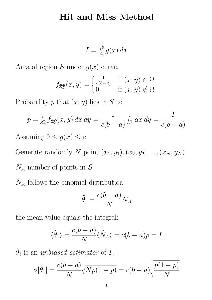
I =

b

a g(x) dx

Area of region S under g(x) curve. fˆ

xˆ y(x, y) =

      

1 c(b−a)

if (x, y) ∈ Ω if (x, y) / ∈ Ω Probability p that (x, y) lies in S is: p =

• Ω fˆ

xˆ y(x, y) dx dy =

1 c(b − a)

• S dx dy =

I c(b − a) Assuming 0 ≤ g(x) ≤ c Generate randomly N point (x1, y1), (x2, y2), ..., (xN, yN) ˆ NA number of points in S ˆ NA follows the binomial distribution ˆ θ1 = c(b − a) N ˆ NA the mean value equals the integral: ˆ θ1 = c(b − a) N ˆ NA = c(b − a)p = I ˆ θ1 is an unbiased estimator of I. σ[ˆ θ1] = c(b − a) N

• Np(1 − p) = c(b − a)
• p(1 − p)

N

1

Replace p by its sample value: ˆ p = ˆ NA/N. I = ˆ θ1 ± σ[ˆ θ1] = c(b − a)ˆ p ± c(b − a)

• ˆ

p(1 − ˆ p) N Relative error: σ[ˆ θ1] < ˆ θ1 > =

• 1 − p

pN decreases for large p. Take c = max(g(x)).

2

subroutine mc1(g,a,b,c,n,r,s) external g na=0 do 1 i=1,n u=ran_u() v=ran_u() if (g(a+(b-a)*u).gt.c*v) na=na+1 1 continue p=real(na)/n r=(b-a)*c*p s=sqrt(p*(1.-p)/n)*c*(b-a) return end

3

Sampling methods: Uniform Sampling I =

b

a g(x) dx

I =

b

a (b − a)g(x)

1 b − a dx ≡ (b − a)

g(x)fˆ

x(x) dx

I = (b − a)Ex[g(x)] ˆ x es ˆ U(a, b): fˆ

x(x) =

    

1 b−a

if a ≤ x ≤ b

• therwise

Sample mean: ˆ µN[g(x)] = 1 N

N

• i=1 g(xi)

r.v. ˆ θ2 = (b − a)ˆ µN from sampling: ˆ θ2 = (b − a) 1 N

N

• i=1 g(xi)

xi, i = 1, 2, ..., N uniformly distributed in the interval [a, b]. θ2 = I I = ˆ θ2 ± σ[ˆ θ2] = ˆ θ2 ± (b − a)σ[g(x)] √ N ˆ σ2

N =

    1

N

N

• i=1 g(xi)2 −

   1

N

N

• i=1 g(xi)

  

2

  

4

subroutine mc2(g,a,b,n,r,s) external g r1=0. s1=0. do 1 i=1,n u=ran_u() g0=g(a+(b-a)*u) r1=r1+g0 s1=s1+g0*g0 1 continue r1=r1/n s1=sqrt((s1/n-r1*r1)/n) r=(b-a)*r1 s=(b-a)*s1 return end

5

Method of Importance Sampling I =

b

a g(x)fˆ x(x) dx

I = Ex[g(x)] ˆ x distributed according fˆ

x(x). Sample mean:

ˆ µN[g(x)] = 1 N

N

• i=1 g(xi)

xi, i = 1, 2, ..., N are values of the r.v. ˆ x distributed according to fˆ

x(x)

Unbiased estimator ˆ µN[g(x)] = I. I = ˆ µN[g(x)] ± σ[ˆ µN[g(x)]] I = ˆ µN[g(x)] ± σ[g(x)] √ N σ2[g(x)] =

fˆ

xg(x)2 dx − (

fˆ

xg(x) dx)2

Use sample variance ˆ σ2

N:

ˆ σ2

N =

    1

N

N

• i=1 g(xi)2 −

   1

N

N

• i=1 g(xi)

  

2

  

How do we generate ˆ xi? If ui is a ˆ U(0, 1) variable, then: xi = F −1

ˆ x (ui)

6

subroutine mc3(g,n,r,s) external g r=0. s=0. do 1 i=1,n x=ran_f() g0=g(x) r=r+g0 s=s+g0*g0 1 continue r=r/n s=sqrt((s/n-r*r)/n) return end

7

Efficiency of an integration method Computer time needed to compute a given integral with a given error ǫ. So far: ǫ = σ √ N t is the computer time needed to add a contribution to the estimator total computer time Nt ∝ tσ2 Relative efficiency of method 1 and 2: e12 = t1σ2

1

t2σ2

2

Uniform sampling is more efficient that hit and miss method. Hit and miss: σ2

1 = c(b − a)I − I2

Uniform sampling: σ2

2 = (b − a)

g(x)2 dx − I2

σ2

1 − σ2 2 = (b − a)

• cI −

g(x)2 dx

• 8

The condition 0 ≤ g(x) ≤ c implies:

g(x)2 dx ≤ c g(x) dx = cI

and σ1 ≥ σ2. Furthermore, in general, t1 > t2, and it follows e12 > 1. Advantages and disadvantages of the Monte-Carlo integration Very singular function n−dimensional integral, with high n

• Ω g(x1, x2, . . . , xn)fˆ

x1...ˆ xn(x1, x2, . . . , xn) dx1 dx2 . . . dxn ≈

1 N

N

• i=1 g(x1, x2, . . . , xn)

(x1, x2, . . . , xn) is a random vector distributed according the probability density function fˆ

x1...ˆ xn(x1, x2, . . . , xn).

Everything is valid for sums:

• i gi =

g(x)fˆ

x(x) dx

by considering a discrete random variable fˆ

x(x) =

• i piδ(x − xi)

9

and gi = g(xi)

10