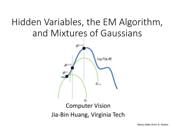
Hidden Variables, the EM Algorithm, and Mixtures of Gaussians - - PowerPoint PPT Presentation

SLIDE 1

Hidden Variables, the EM Algorithm, and Mixtures of Gaussians

Computer Vision Jia-Bin Huang, Virginia Tech

Many slides from D. Hoiem

SLIDE 2

Administrative stuffs

• Final project
• proposal due soon - extended to Oct 29 Monday
• Tips for final project
• Set up several milestones
• Think about how you are going to evaluate
• Demo is highly encouraged
• HW 4 out tomorrow

SLIDE 3

Sample final projects

• State quarter classification
• Stereo Vision - correspondence matching
• Collaborative monocular SLAM for Multiple Robots in an unstructured

environment

• Fight Detection using Convolutional Neural Networks
• Actor Rating using Facial Emotion Recognition
• Fiducial Markers on Bat Tracking Based on Non-rigid Registration
• Im2Latex: Converting Handwritten Mathematical Expressions to Latex
• Pedestrian Detection and Tracking
• Inference with Deep Neural Networks
• Rubik's Cube
• Plant Leaf Disease Detection and Classification
• MBZIRC Challenge-2017
• Multi-modal Learning Scheme for Athlete Recognition System in Long Video
• Computer Vision In Quantitative Phase Imaging
• Aircraft pose estimation for level flight
• Automatic segmentation of brain tumor from MRI images
• Visual Dialog
• PixelDream

SLIDE 4

Superpixel algorithms

• Goal: divide the image into a large number of

regions, such that each regions lie within object boundaries

• Examples
• Watershed
• Felzenszwalb and Huttenlocher graph-based
• Turbopixels
• SLIC

SLIDE 5

Watershed algorithm

SLIDE 6

Watershed segmentation

Image Gradient Watershed boundaries

SLIDE 7

Meyer’s watershed segmentation

• 1. Choose local minima as region seeds
• 2. Add neighbors to priority queue, sorted by value
• 3. Take top priority pixel from queue

1. If all labeled neighbors have same label, assign that label to pixel 2. Add all non-marked neighbors to queue

• 4. Repeat step 3 until finished (all remaining pixels

in queue are on the boundary)

Meyer 1991

Matlab: seg = watershed(bnd_im)

SLIDE 8

Simple trick

• Use Gaussian or median filter to reduce number of

regions

SLIDE 9

Watershed usage

• Use as a starting point for hierarchical segmentation

–Ultrametric contour map (Arbelaez 2006)

• Works with any soft boundaries

–Pb (w/o non-max suppression) –Canny (w/o non-max suppression) –Etc.

SLIDE 10

Watershed pros and cons

• Pros

–Fast (< 1 sec for 512x512 image) –Preserves boundaries

• Cons

–Only as good as the soft boundaries (which may be slow to compute) –Not easy to get variety of regions for multiple segmentations

• Usage

–Good algorithm for superpixels, hierarchical segmentation

SLIDE 11

Felzenszwalb and Huttenlocher: Graph- Based Segmentation

+ Good for thin regions + Fast + Easy to control coarseness of segmentations + Can include both large and small regions

• Often creates regions with strange shapes
• Sometimes makes very large errors

http://www.cs.brown.edu/~pff/segment/

SLIDE 12

Turbo Pixels: Levinstein et al. 2009

http://www.cs.toronto.edu/~kyros/pubs/09.pami.turbopixels.pdf

Tries to preserve boundaries like watershed but to produce more regular regions

SLIDE 13

SLIC (Achanta et al. PAMI 2012)

• 1. Initialize cluster centers on pixel

grid in steps S

• Features: Lab color, x-y position
• 2. Move centers to position in 3x3

window with smallest gradient

• 3. Compare each pixel to cluster

center within 2S pixel distance and assign to nearest

• 4. Recompute cluster centers as

mean color/position of pixels belonging to each cluster

• 5. Stop when residual error is

small

http://infoscience.epfl.ch/record/177415/files/Superpixel_PAMI2011-2.pdf + Fast 0.36s for 320x240 + Regular superpixels + Superpixels fit boundaries

• May miss thin objects
• Large number of superpixels

SLIDE 14

Choices in segmentation algorithms

• Oversegmentation
• Watershed + Structure random forest
• Felzenszwalb and Huttenlocher 2004

http://www.cs.brown.edu/~pff/segment/

• SLIC
• Turbopixels
• Mean-shift
• Larger regions (object-level)
• Hierarchical segmentation (e.g., from Pb)
• Normalized cuts
• Mean-shift
• Seed + graph cuts (discussed later)

SLIDE 15

Multiple segmentations

• Don’t commit to one partitioning
• Hierarchical segmentation
• Occlusion boundaries hierarchy: Hoiem et al.

IJCV 2011 (uses trained classifier to merge)

• Pb+watershed hierarchy: Arbeleaz et al. CVPR

2009

• Selective search: FH + agglomerative clustering
• Superpixel hierarchy
• Vary segmentation parameters
• E.g., multiple graph-based segmentations or

mean-shift segmentations

• Region proposals
• Propose seed superpixel, try to segment out
• bject that contains it

(Endres Hoiem ECCV 2010, Carreira Sminchisescu CVPR 2010)

SLIDE 16

Review: Image Segmentation

• Gestalt cues and principles of
• rganization
• Uses of segmentation
• Efficiency
• Provide feature supports
• Propose object regions
• Want the segmented object
• Segmentation and grouping
• Gestalt cues
• By clustering (k-means, mean-shift)
• By boundaries (watershed)
• By graph (merging , graph cuts)
• By labeling (MRF) <- Next lecture

SLIDE 17

HW 4: SLIC (Achanta et al. PAMI 2012)

• 1. Initialize cluster centers on pixel

grid in steps S

• Features: Lab color, x-y position
• 2. Move centers to position in 3x3

window with smallest gradient

• 3. Compare each pixel to cluster

center within 2S pixel distance and assign to nearest

• 4. Recompute cluster centers as

mean color/position of pixels belonging to each cluster

• 5. Stop when residual error is

small

http://infoscience.epfl.ch/record/177415/files/Superpixel_PAMI2011-2.pdf + Fast 0.36s for 320x240 + Regular superpixels + Superpixels fit boundaries

• May miss thin objects
• Large number of superpixels

SLIDE 18

Today’s Class

• Examples of Missing Data Problems
• Detecting outliers
• Latent topic models
• Segmentation (HW 4, problem 2)
• Background
• Maximum Likelihood Estimation
• Probabilistic Inference
• Dealing with “Hidden” Variables
• EM algorithm, Mixture of Gaussians
• Hard EM

SLIDE 19

Missing Data Problems: Outliers

You want to train an algorithm to predict whether a photograph is attractive. You collect annotations from Mechanical Turk. Some annotators try to give accurate ratings, but others answer randomly. Challenge: Determine which people to trust and the average rating by accurate annotators.

Photo: Jam343 (Flickr)

Annotator Ratings 10 8 9 2 8

SLIDE 20

Missing Data Problems: Object Discovery

You have a collection of images and have extracted regions from them. Each is represented by a histogram of “visual words”. Challenge: Discover frequently occurring object categories, without pre-trained appearance models.

http://www.robots.ox.ac.uk/~vgg/publications/papers/russell06.pdf

SLIDE 21

Missing Data Problems: Segmentation

You are given an image and want to assign foreground/background pixels. Challenge: Segment the image into figure and ground without knowing what the foreground looks like in advance.

Foreground Background

SLIDE 22

Missing Data Problems: Segmentation

Challenge: Segment the image into figure and ground without knowing what the foreground looks like in advance. Three steps: 1. If we had labels, how could we model the appearance of foreground and background?

• Maximum Likelihood Estimation

2. Once we have modeled the fg/bg appearance, how do we compute the likelihood that a pixel is foreground?

• Probabilistic Inference

3. How can we get both labels and appearance models at once?

• Expectation-Maximization (EM) Algorithm

SLIDE 23

Maximum Likelihood Estimation

1. If we had labels, how could we model the appearance

• f foreground and background?

Foreground Background

SLIDE 24

Maximum Likelihood Estimation

 



  

n n N

x p p x x ) | ( argmax ˆ ) | ( argmax ˆ ..

1

   

 

x x

data parameters

SLIDE 25

Maximum Likelihood Estimation

 



  

n n N

x p p x x ) | ( argmax ˆ ) | ( argmax ˆ ..

1

   

 

x x

Gaussian Distribution

 

          

2 2 2 2

2 exp 2 1 ) , | (     

n n

x x p

SLIDE 26

Maximum Likelihood Estimation

መ 𝜄 = argmax𝜄 𝑞 𝐲 𝜄) = argmax𝜄 log 𝑞 𝐲 𝜄) መ 𝜄 = argmax𝜄 ෍

𝑜

log (𝑞 𝑦𝑜 𝜄 ) = argmax𝜄 𝑀(𝜄) 𝑀 𝜄 = −𝑂 2 log 2𝜌 − −𝑂 2 log 𝜏2 − 1 2𝜏2 ෍

𝑜

𝑦𝑜 − 𝜈 2 𝜖𝑀(𝜄) 𝜖𝜈 = 1 𝜏2 ෍

𝑜

𝑦𝑜 − 𝑣 = 0 → ො 𝜈 = 1 𝑂 ෍

𝑜

𝑦𝑜 𝜖𝑀(𝜄) 𝜖𝜏 = 𝑂 𝜏 − 1 𝜏3 ෍

𝑜

𝑦𝑜 − 𝜈 2 = 0 → 𝜏2 = 1 𝑂 ෍

𝑜

𝑦𝑜 − ො 𝜈 2 Log-Likelihood

 

          

2 2 2 2

2 exp 2 1 ) , | (     

n n

x x p

Gaussian Distribution

SLIDE 27

Maximum Likelihood Estimation

 



  

n n N

x p p x x ) | ( argmax ˆ ) | ( argmax ˆ ..

1

   

 

x x

 

          

2 2 2 2

2 exp 2 1 ) , | (     

n n

x x p

Gaussian Distribution





n n

x N 1 ˆ 

 



 

n n

x N

2 2

ˆ 1 ˆ  

SLIDE 28

Example: MLE

>> mu_fg = mean(im(labels)) mu_fg = 0.6012 >> sigma_fg = sqrt(mean((im(labels)-mu_fg).^2)) sigma_fg = 0.1007 >> mu_bg = mean(im(~labels)) mu_bg = 0.4007 >> sigma_bg = sqrt(mean((im(~labels)-mu_bg).^2)) sigma_bg = 0.1007

labels im fg: mu=0.6, sigma=0.1 bg: mu=0.4, sigma=0.1 Parameters used to Generate

SLIDE 29

Probabilistic Inference

2. Once we have modeled the fg/bg appearance, how do we compute the likelihood that a pixel is foreground?

Foreground Background

SLIDE 30

Probabilistic Inference

Compute the likelihood that a particular model generated a sample

component or label

) , | ( 

n n

x m z p 

SLIDE 31

Probabilistic Inference

component or label

   

   | | , ) , | (

n m n n n n

x p x m z p x m z p    Compute the likelihood that a particular model generated a sample

Conditional probability

𝑄 𝐵 𝐶 = 𝑄(𝐵, 𝐶) 𝑄(𝐶)

SLIDE 32

Probabilistic Inference

component or label

   

   | | , ) , | (

n m n n n n

x p x m z p x m z p   

   



  

k k n n m n n

x k z p x m z p   | , | , Compute the likelihood that a particular model generated a sample

Marginalization

𝑄 𝐵 = ෍

𝑙

𝑄(𝐵, 𝐶 = 𝑙)

SLIDE 33

Probabilistic Inference

component or label

   

   | | , ) , | (

n m n n n n

x p x m z p x m z p   

       



    

k k n k n n m n m n n

k z p k z x p m z p m z x p     | , | | , |

   



  

k k n n m n n

x k z p x m z p   | , | , Compute the likelihood that a particular model generated a sample

Joint distribution

𝑄 𝐵, 𝐶 = P B P(A|B)

SLIDE 34

Example: Inference

>> pfg = 0.5; >> px_fg = normpdf(im, mu_fg, sigma_fg); >> px_bg = normpdf(im, mu_bg, sigma_bg); >> pfg_x = px_fg*pfg ./ (px_fg*pfg + px_bg*(1-pfg));

im fg: mu=0.6, sigma=0.1 bg: mu=0.4, sigma=0.1 Learned Parameters p(fg | im)

SLIDE 35

Dealing with Hidden Variables

3. How can we get both labels and appearance parameters at once?

Foreground Background

SLIDE 36

Mixture of Gaussians

 

m m m n m

x                

2 2 2

2 exp 2 1

 

 

m m m n n n n

m z x p m z x p    , , | , , , | ,

2 2

   π σ μ

  



m n m m n

m z p x p    | , |

2

 

mixture component

 

 



 

m m m m n n n

m z x p x p    , , | , , , |

2 2 π

σ μ

component prior component model parameters

SLIDE 37

Mixture of Gaussians

With enough components, can represent any probability density function

• Widely used as general purpose pdf estimator

SLIDE 38

Segmentation with Mixture of Gaussians

Pixels come from one of several Gaussian components

• We don’t know which pixels come from which

components

• We don’t know the parameters for the components

Problem:

• Estimate the parameters of the

Gaussian Mixture Model. What would you do?

SLIDE 39

Simple solution

• 1. Initialize parameters
• 2. Compute the probability of each hidden variable

given the current parameters

• 3. Compute new parameters for each model,

weighted by likelihood of hidden variables

• 4. Repeat 2-3 until convergence

SLIDE 40

Mixture of Gaussians: Simple Solution

• 1. Initialize parameters
• 2. Compute likelihood of hidden variables for

current parameters

• 3. Estimate new parameters for each model,

weighted by likelihood ) , , , | (

) ( ) ( 2 ) ( t t t n n nm

x m z p π σ μ     



 n n nm n nm t m

x    1 ˆ

) 1 (

 

 

 

 n m n nm n nm t m

x

2 ) 1 ( 2

ˆ 1 ˆ    

N

n nm t m







 

) 1 (

ˆ

SLIDE 41

Expectation Maximization (EM) Algorithm

 

     



z

z x  



| , log argmax ˆ p

Goal:

 

   

 

X f X f E E 

Jensen’s Inequality Log of sums is intractable

See here for proof: www.stanford.edu/class/cs229/notes/cs229-notes8.ps

for concave functions f(x) (so we maximize the lower bound!)

SLIDE 42

Expectation Maximization (EM) Algorithm

• 1. E-step: compute
• 2. M-step: solve

   

 

    



) ( , |

, | | , log | , log E

) (

t x z

p p p

t

  



x z z x z x

z





    



) ( ) 1 (

, | | , log argmax

t t

p p   



x z z x

z







 

     



z

z x  



| , log argmax ˆ p

Goal:

SLIDE 43

Expectation Maximization (EM) Algorithm

• 1. E-step: compute
• 2. M-step: solve

   

 

    



) ( , |

, | | , log | , log E

) (

t x z

p p p

t

  



x z z x z x

z





    



) ( ) 1 (

, | | , log argmax

t t

p p   



x z z x

z







 

     



z

z x  



| , log argmax ˆ p

Goal:

 

   

 

X f X f E E 

log of expectation of P(x|z) expectation of log of P(x|z)

SLIDE 44

EM for Mixture of Gaussians - derivation

 



           

m m m m n m

x    

2 2 2 exp

2 1

 

 



 

m m m m n n n

m z x p x p    , , | , , , |

2 2 π

σ μ

1. E-step: 2. M-step:

          



) ( , |

, | | , log | , log E

) (

t x z

p p p

t

  



x z z x z x

z





    



) ( ) 1 (

, | | , log argmax

t t

p p   



x z z x

z







SLIDE 45

EM for Mixture of Gaussians

 



           

m m m m n m

x    

2 2 2 exp

2 1

 

 



 

m m m m n n n

m z x p x p    , , | , , , |

2 2 π

σ μ

1. E-step: 2. M-step:

          



) ( , |

, | | , log | , log E

) (

t x z

p p p

t

  



x z z x z x

z





    



) ( ) 1 (

, | | , log argmax

t t

p p   



x z z x

z







) , , , | (

) ( ) ( 2 ) ( t t t n n nm

x m z p π σ μ     



 n n nm n nm t m

x    1 ˆ

) 1 (

 

 

 

 n m n nm n nm t m

x

2 ) 1 ( 2

ˆ 1 ˆ    

N

n nm t m







 

) 1 (

ˆ

SLIDE 46

EM algorithm - derivation

http://lasa.epfl.ch/teaching/lectures/ML_Phd/Notes/GP-GMM.pdf

SLIDE 47

EM algorithm – E-Step

SLIDE 48

EM algorithm – E-Step

SLIDE 49

EM algorithm – M-Step

SLIDE 50

EM algorithm – M-Step

Take derivative with respect to 𝜈𝑚

SLIDE 51

EM algorithm – M-Step

Take derivative with respect to σ𝑚

−1

SLIDE 52

EM Algorithm for GMM

SLIDE 53

EM Algorithm

• Maximizes a lower bound on the data likelihood at

each iteration

• Each step increases the data likelihood
• Converges to local maximum
• Common tricks to derivation
• Find terms that sum or integrate to 1
• Lagrange multiplier to deal with constraints

SLIDE 54

Convergence of EM Algorithm

SLIDE 55

EM Demos

• Mixture of Gaussian demo
• Simple segmentation demo

SLIDE 56

“Hard EM”

• Same as EM except compute z* as most likely values for

hidden variables

• K-means is an example
• Advantages
• Simpler: can be applied when cannot derive EM
• Sometimes works better if you want to make hard predictions

at the end

• But
• Generally, pdf parameters are not as accurate as EM

SLIDE 57

Missing Data Problems: Outliers

You want to train an algorithm to predict whether a photograph is attractive. You collect annotations from Mechanical Turk. Some annotators try to give accurate ratings, but others answer randomly. Challenge: Determine which people to trust and the average rating by accurate annotators.

Photo: Jam343 (Flickr)

Annotator Ratings 10 8 9 2 8

SLIDE 58

Next class

• MRFs and Graph-cut Segmentation
• Think about your final projects (if not done already)